In the diverse realm of mathematics, the term ‘how to solve an equation graphically’ refers to a technique that leverages the visual allure and intuitive nature of graphs.
In this article, we’ll explore the nuances of this method, guiding you through the steps to transform convoluted equations into comprehensible visual narratives.
How to Solve an Equation Graphically
To solve an equation graphically, the equation is represented using graphs on a coordinate plane, and the solution is often where the graph intersects a given axis.
With the aim of identifying solutions based on visual representation an equation or a system of equations is represented by graphs on a coordinate plane.
For a system of equations, the solution is the point or points where the graphs of the equations intersect. This method provides a visual approach to problem-solving and can be especially useful for understanding the nature and number of solutions, as well as for equations that are challenging to solve algebraically.
Example
Trigonometric Equation: y = sin(x)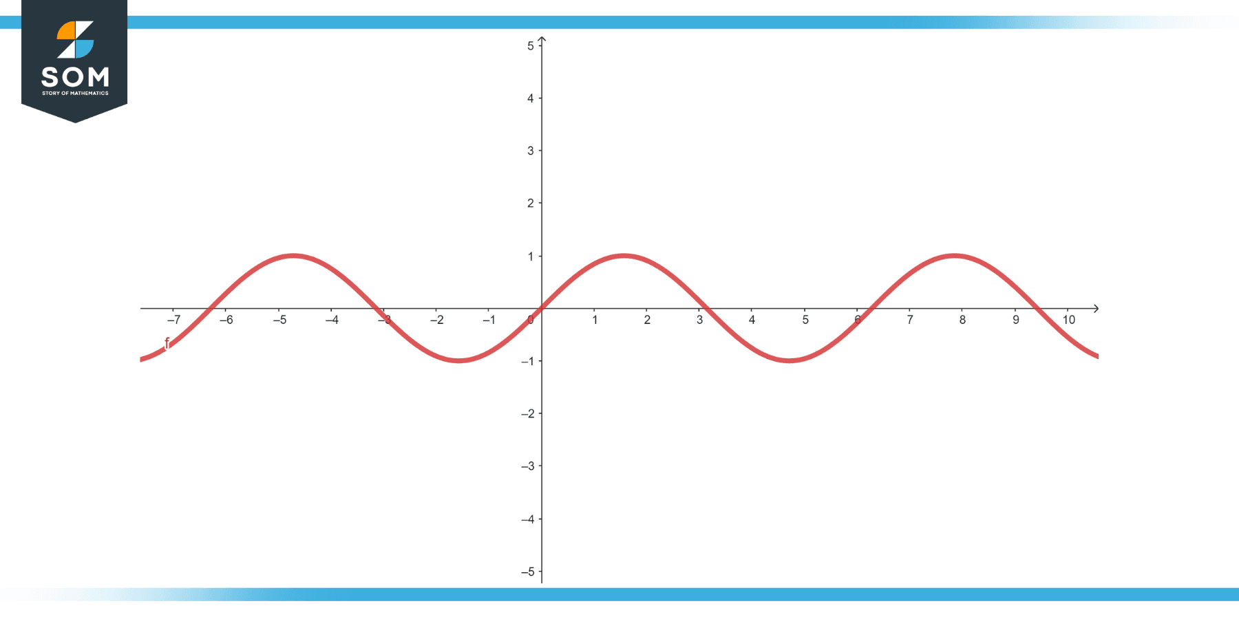
Figure-1.
To find where y = 0, graph the sine function. The solutions in one period (0 to 2π) are x = π and x = 2π.
Properties
Solving an equation graphically involves interpreting points, intersections, and behaviors of curves and lines on a graph. While this method isn’t guided by strict “properties” like some algebraic techniques, there are key characteristics and principles to consider:
Intersections as Solutions
- For a single equation, points where the curve (or line) intersects the x-axis represent its roots or solutions.
- For a system of equations, the points where the graphs intersect represent the solutions to the system.
Number of Solutions
- The number of intersections denotes how many solutions exist. For instance, a quadratic function can have 0, 1, or 2 solutions depending on whether its graph intersects the x-axis zero times, once, or twice, respectively.
Nature of Solutions
- Real vs Imaginary Solutions: If a graph does not intersect the x-axis, its equation might have complex or imaginary solutions.
- Unique vs Infinite Solutions: For a system of linear equations, if two lines are coincident (one on top of the other), there are infinite solutions. If they are parallel, there’s no solution.
Continuous vs Discontinuous Graphs
- Some functions have breaks or holes. It’s crucial to recognize that a point of discontinuity is not an intersection with the x-axis and therefore is not a solution.
Dependent and Independent Variables
- Typically, the x-axis represents the independent variable and the y-axis represents the dependent variable. However, this can change based on the context or specific mathematical scenario.
Limitations and Approximations
- Graphical solutions can be approximations. If high precision is required, further algebraic or numerical methods may be needed.
- The scale and accuracy of the graphing tool (whether it’s software or graph paper) can influence the perceived solution.
Domain and Range
- The domain represents all possible input (x) values. The range represents all potential output (y) values. When graphing, it’s crucial to consider the domain of the equation, as it affects the portion of the graph visible or relevant to the solution.
Asymptotes
- Vertical asymptotes can be indicative of values that the function approaches but never reaches. They can signal undefined points in the function.
- Horizontal asymptotes provide insight into the function’s behavior as the independent variable approaches positive or negative infinity.
Symmetry
- Equations can have symmetry about the y-axis, x-axis, or origin. Recognizing symmetry can simplify the graphing process and help identify solutions.
Behavior at Intersections
- Not every intersection guarantees a solution to every system. For instance, in inequalities, one is often interested in areas of overlap or non-overlap rather than mere intersections.
Exercise
Example 1
Linear Equation
Equation: y = 2x + 1
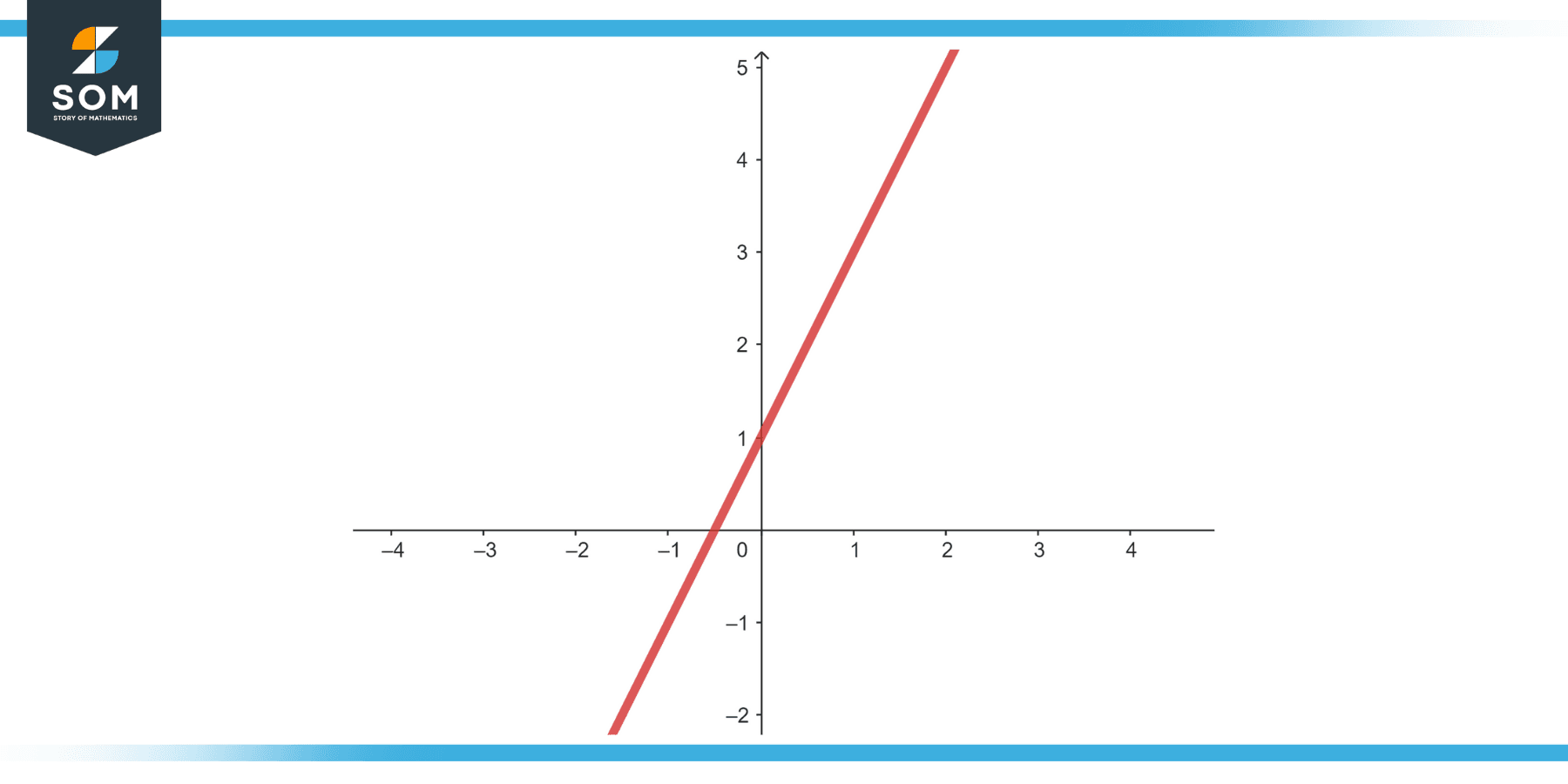
Figure-2.
Solution
Graph the line. The x-intercept (where y = 0) will give the solution for x. Graphically, the line will cut the x-axis at x = -0.5. Therefore, the solution is x = -0.5.
Example 2
Quadratic Equation
Equation: y = $x^2$ – 4 * x + 3
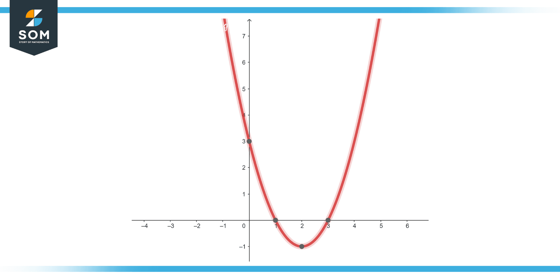
Figure-3.
Solution
The solutions are the x-values where the graph touches or crosses the x-axis. Factorizing, we get: y = (x – 3)(x – 1). Graphically, this parabola will intersect the x-axis at x-values 1 and 3.
Example 3
Cubic Equation
Equation: y = $x^3 – 6 * x^2$ + 11 * x – 6
Solution
The graph will cross the x-axis wherever the equation has real roots. Factoring, we get y = (x – 1)(x – 2)(x – 3). So, graphically, the solutions are x-values 1, 2, and 3.
Applications
Mathematics
- Teaching: Graphical solutions help in pedagogy, enabling students to visualize complex concepts, especially in algebra and calculus.
- Study of Functions: Analysing the behavior of functions, such as polynomials, trigonometric functions, and exponentials, is often facilitated by graphical representation.
Physics
- Kinematics: Graphs of position, velocity, and acceleration versus time can be used to solve for specific moments when certain conditions are met, like when velocity is zero.
- Equilibrium Problems: Graphs can depict the resultant of forces or torques to determine equilibrium points.
Economics
- Supply and Demand: Equilibrium prices and quantities are found at the intersection of the supply and demand curves.
- Cost Analysis: Identifying break-even points by plotting cost and revenue curves.
Engineering
- Control Systems: Root locus plots help engineers design and understand the behavior of control systems.
- Optimization Problems: Engineers might use graphical methods to visualize constraints and identify feasible solutions.
Biology and Medicine
- Population Dynamics: Growth curves, predator-prey models, and logistic models can be graphically analyzed to understand and predict population trends.
- Dose-Response Curves: In pharmacology, these curves illustrate the effect of different drug dose levels, helping in determining optimal dosages.
Environmental Science
- Pollution Studies: Plotting the concentration of pollutants against time or distance can help identify sources or sinks of pollution.
- Climate Studies: Graphical methods can be employed to analyze temperature changes, greenhouse gas concentrations, and more.
Geography and Geology
- Topographic Analysis: Contour plots give insights into terrains, helping in tasks ranging from urban planning to geological studies.
- Seismic Studies: Graphical plots of seismic waves help in determining the epicenter and understanding the depth of earthquakes.
Computer Science
- Algorithm Analysis: Graphs can depict how the runtime of an algorithm varies with input size, aiding in performance optimization.
- Data Visualization: Visualization tools employ graphical techniques to represent complex data sets, helping in data interpretation and decision-making.
Finance
- Risk Analysis: Plotting potential investment returns against risks can help investors make informed decisions.
- Time Series Analysis: Stock prices, indices, or other financial metrics can be graphed over time to detect patterns, trends, or anomalies.
Social Sciences
- Sociological Trends: Graphs can represent trends like migration, urbanization, or demographic changes.
- Psychology: In experimental psychology, graphical methods can be used to illustrate patterns or trends in data, such as response times or behavioral patterns.
All images were created with GeoGebra