JUMP TO TOPIC

In this article, we dive deep into the heart of the orthogonal complement, exploring its definition, properties, and applications. Whether you’re a mathematician seeking to strengthen your understanding or a curious reader drawn towards the enchanting world of linear algebra, this comprehensive guide on the orthogonal complement will illuminate the torchlight.
Definition of Orthogonal Complement
In linear algebra, the orthogonal complement of a subspace W of a vector space V equipped with an inner product, such as the Euclidean space $R^n$, is the set of all vectors in V that are orthogonal to every vector in W.
If you take any vector v from the orthogonal complement and any vector w from W, their inner product will be zero. In other words, v and w are orthogonal.
In mathematical notation, if W is a subspace of V, the orthogonal complement of W is usually denoted as W⊥ (W perp). It is defined as:
W⊥ = { v ∈ V : <v, w> = 0 for all w ∈ W }
Here, “< , >” denotes the inner product of two vectors.
So, the orthogonal complement of W consists of all vectors in V that are perpendicular (or orthogonal) to the vectors in W. This is a very useful concept in many areas of mathematics and its applications, such as in computer graphics, machine learning, and physics.
Figure-1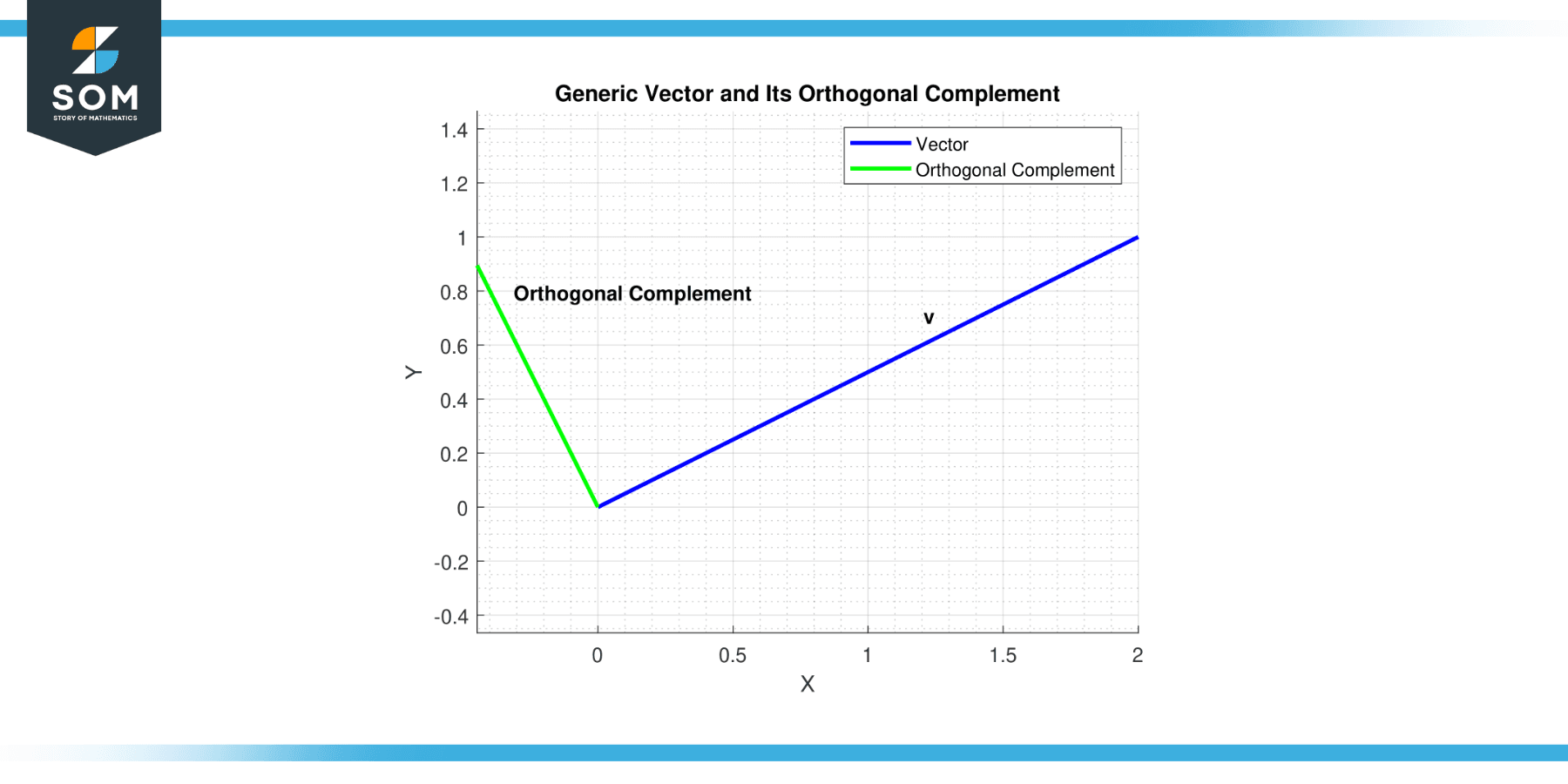 .
.
Properties
Orthogonal complements in vector spaces possess several important properties, making them a critical tool in linear algebra and its applications. These properties directly result from the definitions and axioms of vector spaces and inner products. Here are a few of them:
Non-Negativity
The orthogonal complement of a subspace is always a subspace of the original vector space. This means it is closed under addition and scalar multiplication and contains the zero vector.
Orthogonality
Every vector in the orthogonal complement is orthogonal (perpendicular) to every vector in the original subspace. In other words, the inner product of any vector in the orthogonal complement with any vector in the original subspace is zero.
Self-Orthogonal Complement
The orthogonal complement of a subspace is the original subspace itself (given the subspace and its complement are both finite-dimensional). This property is represented in mathematical notation as (W⊥)⊥ = W.
Zero Intersection
The intersection of a subspace and its orthogonal complement is the zero vector, i.e., W ∩ W⊥ = {0}.
Whole Space
A subspace and its orthogonal complement span the whole vector space in a finite-dimensional vector space. This is mathematically represented as V = W ⊕ W⊥, where ⊕ denotes the direct sum.
Dimensionality
For finite-dimensional spaces, the dimension of a subspace plus its orthogonal complement is equal to the dimension of the entire vector space. This is known as the dimension theorem for vector spaces.
Orthogonal to Itself
If a subspace is orthogonal to itself, i.e., W = W⊥, it must be the zero subspace or the entire vector space.
These properties provide a robust framework for manipulating and understanding orthogonal complements in various contexts, including solving systems of linear equations, orthogonal projections, the Gram-Schmidt process, and more.
Evaluating the Orthogonal Complement
The process of finding orthogonal components relies heavily on the concept of projection. The projection of a vector onto another vector provides the component of the first vector that lies along the second.
The orthogonal complement to that projection is the component of the first vector orthogonal to the second. Here’s a step-by-step process to find the orthogonal component of a vector v concerning another vector u:
Step 1
Start with vectors u and v in the same vector space.
Step 2
Calculate the projection of v onto u. The projection of v onto u is given by the formula:
proj_u(v) = ((v·u) / ||u||²) * u
where v·u denotes the dot product of v and u, and ||u|| denotes the norm (length) of u. This results in a new vector that lies along u.
Step 3
Subtract the projection from v. The difference v - proj_u(v) is the orthogonal component v with respect to u. This vector is orthogonal to u.
Let’s look at an example in R²:
Suppose v = (4, 3) and u = (2, 2). We want to find the orthogonal component of v with respect to u.
Step 1
We have our vectors v = (4, 3) and u = (2, 2).
Step 2
Calculate the projection of v onto u:
proj_u(v) = ((v·u) / ||u||²) * u
proj_u(v) = ((4*2 + 3*2) / (2² + 2²)) * (2, 2)
proj_u(v) = (14/8) * (2, 2)
proj_u(v) = (3.5, 3.5)
Step 3
Subtract the projection from v to get the orthogonal component:
v - proj_u(v) = (4, 3) - (3.5, 3.5)
v - proj_u(v) = (0.5, -0.5)
So, the orthogonal component of v = (4, 3) with respect to u = (2, 2) is (0.5, -0.5). As you can check, the dot product of (0.5, -0.5) and (2, 2) is zero, confirming that these vectors are indeed orthogonal.
Exercise
Example 1
In R³, consider the subspace W spanned by the vector (1, 1, 0). The orthogonal complement W⊥ will be spanned by vectors orthogonal to (1, 1, 0), such as (-1, 1, 0) and (0, 0, 1).
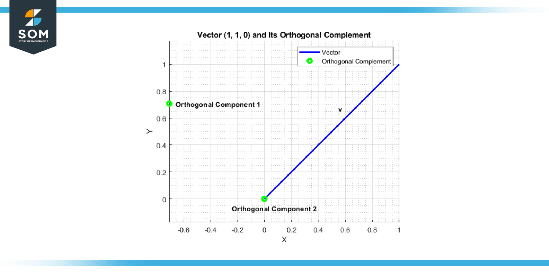
Figure-2.
Example 2
In R², consider the subspace W spanned by the vector (3, 4). The orthogonal complement W⊥ will be spanned by any vector orthogonal to (3, 4), such as (-4, 3).
Example 3
In R³, consider the subspace W spanned by the vectors (1, 0, 0) and (0, 1, 0). The orthogonal complement W⊥ will be spanned by the vector (0, 0, 1), which is orthogonal to both (1, 0, 0) and (0, 1, 0).
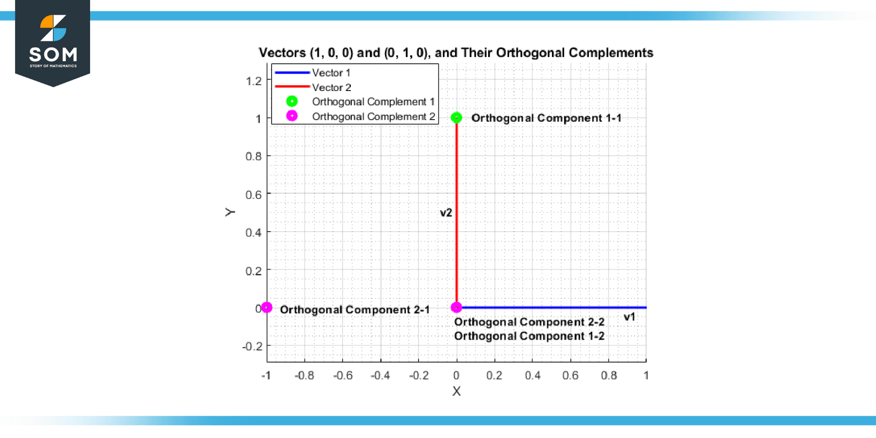
Figure-3.
Example 4
In R², consider the subspace W consisting of the zero vector only (i.e., {0}). The orthogonal complement W⊥ is the entire space R² since every vector in R² is orthogonal to the zero vector.
Example 5
In R², consider the subspace W = R². The orthogonal complement W⊥ is the zero subspace {0} since only the zero vector is orthogonal to every vector in R².
Example 6
In R³, consider the subspace W spanned by the vectors (1, 2, 3) and (4, 5, 6).
A vector v = (x, y, z) is in W⊥ if it’s orthogonal to both (1, 2, 3) and (4, 5, 6), i.e., if x + 2y + 3z = 0 and 4x + 5y + 6z = 0. Solving these gives the orthogonal complement W⊥ as the set of all scalar multiples of (-1, 2, -1).
Example 7
In R⁴, consider the subspace W spanned by the vectors (1, 0, 0, 0), (0, 1, 0, 0), and (0, 0, 1, 0). The orthogonal complement W⊥ will be spanned by the vector (0, 0, 0, 1), which is orthogonal to all vectors in W.
Example 8
In R³, consider the subspace W spanned by the vectors (1, 2, 0) and (2, -1, 0).
A vector v = (x, y, z) is in W⊥ if it’s orthogonal to both (1, 2, 0) and (2, -1, 0), i.e., if x + 2y = 0 and 2x – y = 0. Solving these gives the orthogonal complement W⊥ as the set of all scalar multiples of (0, 0, 1).
Applications
The concept of the orthogonal complement has widespread applications across numerous fields where mathematics, particularly linear algebra, comes into play. Here are some of the areas where it proves useful:
Machine Learning and Data Science
In machine learning, orthogonal complements are used in techniques like Principal Component Analysis (PCA) for dimensionality reduction. PCA identifies the axes in the feature space along which the data varies the most. These axes are orthogonal (perpendicular) to each other, forming an orthogonal complement to the remaining, less significant directions in the data.
Physics
In physics, especially in quantum mechanics, the concept of orthogonal complements is used in Hilbert spaces to describe orthogonal states mutually exclusive. This is important for understanding the behavior and properties of quantum systems.
Computer Graphics and Vision
Orthogonal complements are used in techniques for computing projections of points onto a line or a plane. This is extremely important in 3D computer graphics and computer vision, where objects are often transformed and projected onto different planes for viewing and rendering.
Signal Processing
In digital signal processing, the concept of orthogonality is central to the operation of separating signals from noise or separating multiple signals from each other. Here, orthogonal complements can often be used to isolate the component of a signal that’s orthogonal to the noise.
Engineering
In control theory (a part of engineering), a system’s controllable and uncontrollable subspaces are orthogonal complements of each other. Understanding these can help design control systems like cars, planes, or electronics.
Economics and Finance
In portfolio theory, the risk of a portfolio can be decomposed into systematic and unsystematic risks, which are orthogonal to each other. Similarly, in econometrics, the error term in regression is assumed to be orthogonal to the explanatory variables, helping find the best linear unbiased estimator.
All images were created with GeoGebra and MATLAB.