Solving initial value problems (IVPs) is an important concept in differential equations. Like the unique key that opens a specific door, an initial condition can unlock a unique solution to a differential equation.
As we dive into this article, we aim to unravel the mysterious process of solving initial value problems in differential equations. This article offers an immersive experience to newcomers intrigued by calculus’s wonders and experienced mathematicians looking for a comprehensive refresher.
Solving the Initial Value Problem
To solve an initial value problem, integrate the given differential equation to find the general solution. Then, use the initial conditions provided to determine the specific constants of integration.
An initial value problem (IVP) is a specific problem in differential equations. Here is the formal definition. An initial value problem is a differential equation with a specified value of the unknown function at a given point in the domain of the solution.
More concretely, an initial value problem is typically written in the following form:
dy/dt = f(t, y) with y(t₀) = y₀
Here:
- dy/dt = f(t, y) is the differential equation, which describes the rate of change of the function y with respect to the variable t.
- t₀ is the given point in the domain, often time in many physical problems.
- y(t₀) = y₀ is the initial condition, which specifies the value of the function y at the point t₀.
An initial value problem aims to find the function y(t) that satisfies both the differential equation and the initial condition. The solution y(t) to the IVP is not just any solution to the differential equation, but specifically, the one which passes through the point (t₀, y₀) on the (t, y) plane.
Because the solution of a differential equation is a family of functions, the initial condition is used to find the particular solution that satisfies this condition. This differentiates an initial value problem from a boundary value problem, where conditions are specified at multiple points or boundaries.
Example
Solve the IVP y’ = 1 + y^2, y(0) = 0.
Solution
This is a standard form of a first-order non-linear differential equation known as the Riccati equation. The general solution is y = tan(t + C).
Applying the initial condition y(0) = 0, we get:
0 = tan(0 + C)
So, C = 0.
The solution to the IVP is then y = tan(t).
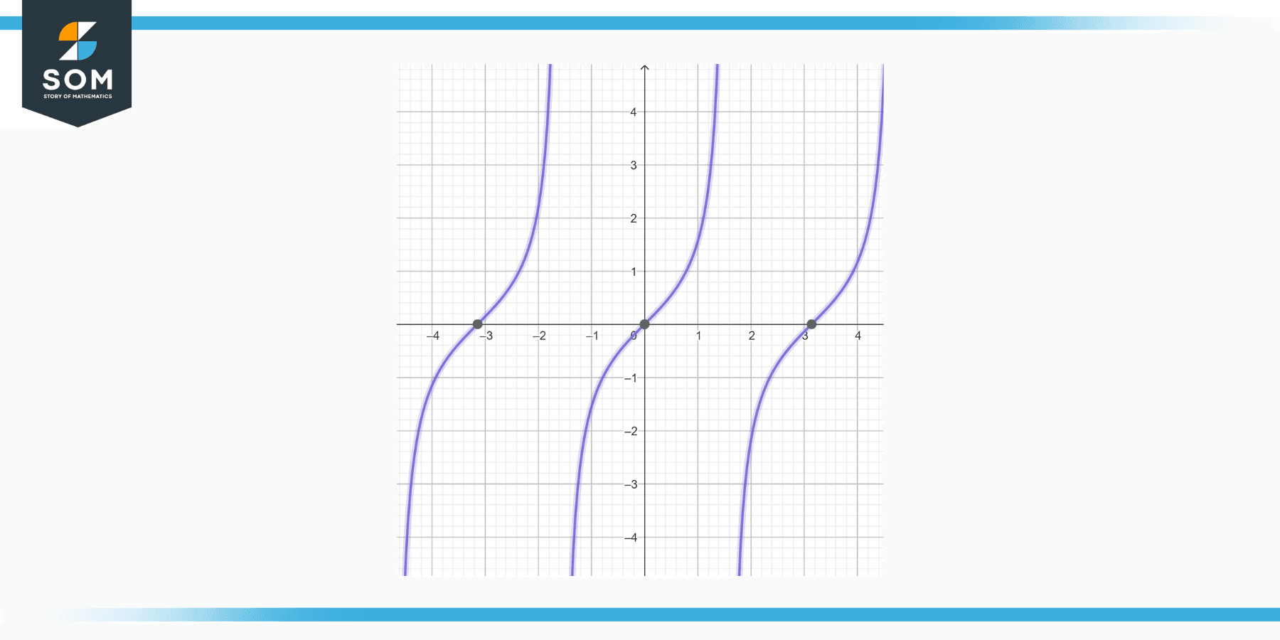
Figure-1.
Properties
Existence and Uniqueness
According to the Existence and Uniqueness Theorem for ordinary differential equations (ODEs), if the function f and its partial derivative with respect to y are continuous in some region of the (t, y)-plane that includes the initial condition (t₀, y₀), then there exists a unique solution y(t) to the IVP in some interval about t = t₀.
In other words, given certain conditions, we are guaranteed to find exactly one solution to the IVP that satisfies both the differential equation and the initial condition.
Continuity and Differentiability
If a solution exists, it will be a function that is at least once differentiable (since it must satisfy the given ODE) and, therefore, continuous. The solution will also be differentiable as many times as the order of the ODE.
Dependence on Initial Conditions
Small changes in the initial conditions can result in drastically different solutions to an IVP. This is often called “sensitive dependence on initial conditions,” a characteristic feature of chaotic systems.
Local vs. Global Solutions
The Existence and Uniqueness Theorem only guarantees a solution in a small interval around the initial point t₀. This is called a local solution. However, under certain circumstances, a solution might extend to all real numbers, providing a global solution. The nature of the function f and the differential equation itself can limit the interval of the solution.
Higher Order ODEs
For higher-order ODEs, you will have more than one initial condition. For an n-th order ODE, you’ll need n initial conditions to find a unique solution.
Boundary Behavior
The solution to an IVP may behave differently as it approaches the boundaries of its validity interval. For example, it might diverge to infinity, converge to a finite value, oscillate, or exhibit other behaviors.
Particular and General Solutions
The general solution of an ODE is a family of functions that represent all solutions to the ODE. By applying the initial condition(s), we narrow this family down to one solution that satisfies the IVP.
Applications
Solving initial value problems (IVPs) is fundamental in many fields, from pure mathematics to physics, engineering, economics, and beyond. Finding a specific solution to a differential equation given initial conditions is essential in modeling and understanding various systems and phenomena. Here are some examples:
Physics
IVPs are used extensively in physics. For example, in classical mechanics, the motion of an object under a force is determined by solving an IVP using Newton’s second law (F=ma, a second-order differential equation). The initial position and velocity (the initial conditions) are used to find a unique solution that describes the object’s motion.
Engineering
IVPs appear in many engineering problems. For instance, in electrical engineering, they are used to describe the behavior of circuits containing capacitors and inductors. In civil engineering, they are used to model the stress and strain in structures over time.
Biology and Medicine
In biology, IVPs are used to model populations’ growth and decay, the spread of diseases, and various biological processes such as drug dosage and response in pharmacokinetics.
Economics and Finance
Differential equations model various economic processes, such as capital growth over time. Solving the accompanying IVP gives a specific solution that models a particular scenario, given the initial economic conditions.
Environmental Science
IVPs are used to model the change in populations of species, pollution levels in a particular area, and the diffusion of heat in the atmosphere and oceans.
Computer Science
In computer graphics, IVPs are used in physics-based animation to make objects move realistically. They’re also used in machine learning algorithms, like neural differential equations, to optimize parameters.
Control Systems
In control theory, IVPs describe the time evolution of systems. Given an initial state, control inputs are designed to achieve a desired state.
Exercise
Example 1
Solve the IVP y’ = 2y, y(0) = 1.
Solution
The given differential equation is separable. Separating variables and integrating, we get:
∫dy/y = ∫2 dt
ln|y| = 2t + C
or
y = $e^{(2t+C)}$
= $e^C * e^{(2t)}$
Now, apply the initial condition y(0) = 1:
1 = $e^C * e^{(2*0)}$
1 = $e^C$
so:
C = ln
1 = 0
The solution to the IVP is y = e^(2t).
Example 2
Solve the IVP y’ = -3y, y(0) = 2.
Solution
The general solution is y = Ce^(-3t). Apply the initial condition y(0) = 2 to get:
2 = C $e^{(-3*0)}$
2 = C $e^0$
2 = C
So, C = 2, and the solution to the IVP is y = 2e^(-3t).
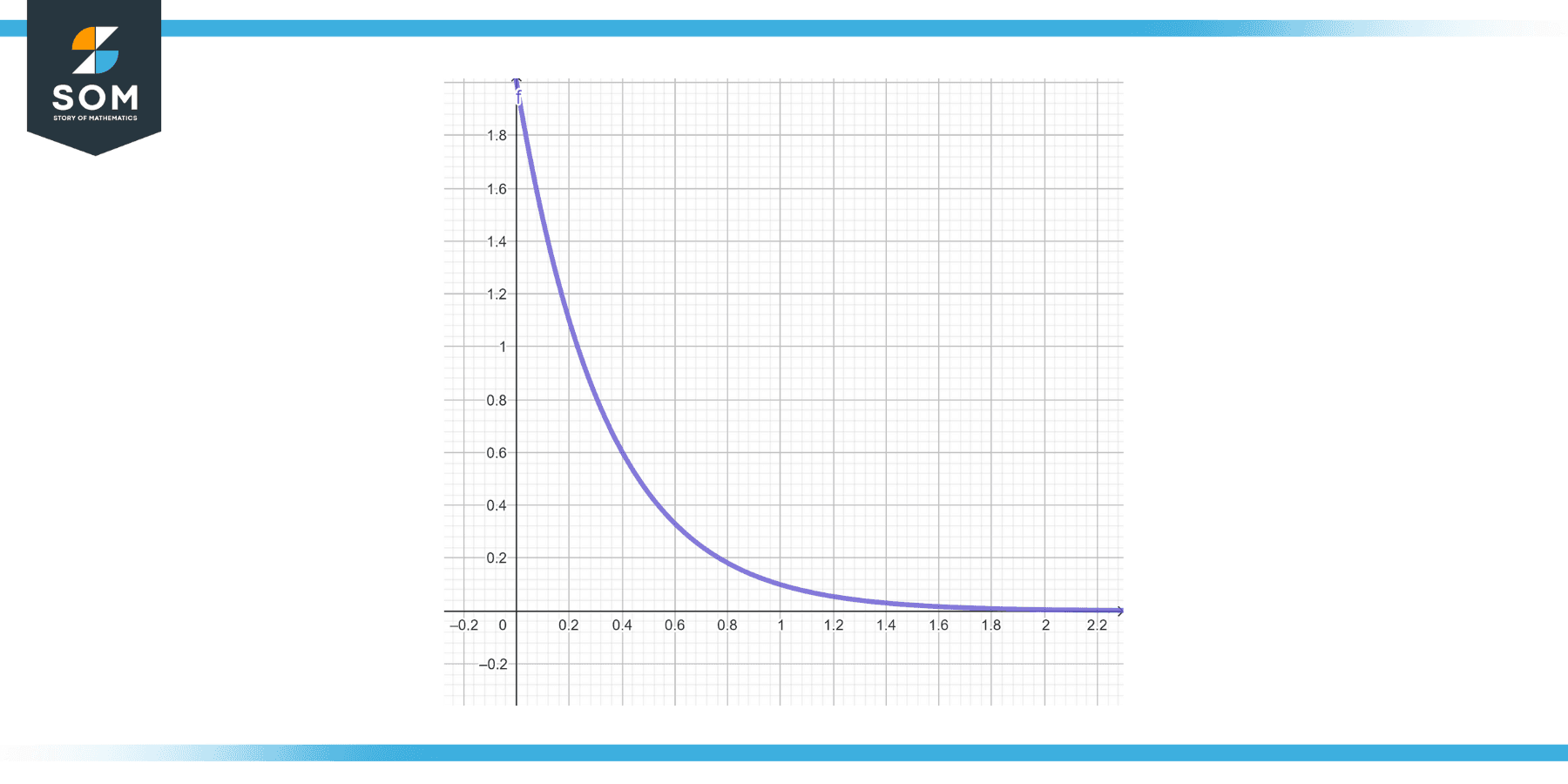
Figure-2.
Example 3
Solve the IVP y’ = y^2, y(1) = 1.
Solution
This is also a separable differential equation. We separate variables and integrate them to get:
∫$dy/y^2$ = ∫dt,
1/y = t + C.
Applying the initial condition y(1) = 1, we find C = -1. So the solution to the IVP is -1/y = t – 1, or y = -1/(t – 1).
Example 4
Solve the IVP y” – y = 0, y(0) = 0, y'(0) = 1.
Solution
This is a second-order linear differential equation. The general solution is y = A sin(t) + B cos(t).
The first initial condition y(0) = 0 gives us:
0 = A0 + B1
So, B = 0.
The second initial condition y'(0) = 1 gives us:
1 = A cos(0) + B*0
So, A = 1.
The solution to the IVP is y = sin(t).
Example 5
Solve the IVP y” + y = 0, y(0) = 1, y'(0) = 0.
Solution
This is also a second-order linear differential equation. The general solution is y = A sin(t) + B cos(t).
The first initial condition y(0) = 1 gives us:
1 = A0 + B1
So, B = 1.
The second initial condition y'(0) = 0 gives us:
0 = A cos(0) – B*0
So, A = 0.
The solution to the IVP is y = cos(t).
Example 6
Solve the IVP y” = 9y, y(0) = 1, y'(0) = 3.
Solution
The differential equation can be rewritten as y” – 9y = 0. The general solution is y = A $ e^{(3t)} + B e^{(-3t)}$.
The first initial condition y(0) = 1 gives us:
1 = A $e^{(30)}$ + B $e^{(-30)}$
= A + B
So, A + B = 1.
The second initial condition y'(0) = 3 gives us:
3 = 3A $e^{30} $ – 3B $e^{-30}$
= 3A – 3B
So, A – B = 1.
We get A = 1 and B = 0 to solve these two simultaneous equations. So, the solution to the IVP is y = $e^{(3t)}$.
Example 7
Solve the IVP y” + 4y = 0, y(0) = 0, y'(0) = 2.
Solution
The differential equation is a standard form of a second-order homogeneous differential equation. The general solution is y = A sin(2t) + B cos(2t).
The first initial condition y(0) = 0 gives us:
0 = A0 + B1
So, B = 0.
The second initial condition y'(0) = 2 gives us:
2 = 2A cos(0) – B*0
So, A = 1.
The solution to the IVP is y = sin(2t).
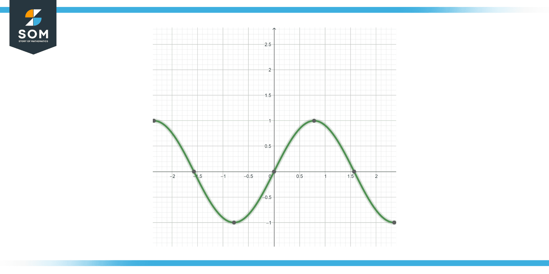
Figure-3.
All images were created with GeoGebra.