This article aims to illuminate the normal line, demystifying their theoretical origins, practical applications, and the sublime beauty inherent in their geometric simplicity.
Definition of the Normal Line
In geometry, the normal line is perpendicular to a given line, plane, or surface at a specific point of contact. When the context involves a curve or a surface, the normal line is typically associated with the tangent line or plane at that point.
For a curve in a two-dimensional space, the normal line is a straight line perpendicular to the tangent line at a particular point on the curve. For a three-dimensional surface, the normal line, often referred to as the ‘normal vector‘ or simply the ‘normal,’ is a vector perpendicular to the tangent plane at a particular point on the surface.
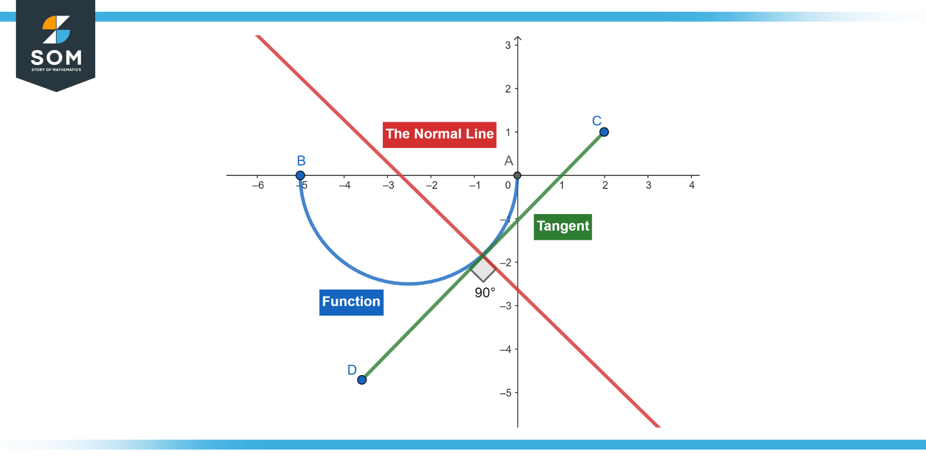
Figure-1.
Properties of the Normal Line
Perpendicular to the Tangent
The normal line is always perpendicular to the tangent line or plane at any given point on a curve or surface. This is the defining property of a normal line.
Unique Direction
In a two-dimensional (2D) plane, only one unique normal line exists for a given point on a curve. This is because the normal line is perpendicular to the tangent line, which is also unique at that point.
However, in three-dimensional (3D) space, for a given point on a surface, the normal line can point in two opposite directions since it is perpendicular to an entire plane, the tangent plane.
Dependent on the Point of Contact
The normal line depends on the point of contact on the curve or surface. Changing the point of contact will generally result in a different normal line.
The magnitude of the Normal Vector
When dealing with normal vectors (normal lines in 3D), the normal vector’s magnitude (or length) is not standardized. It can be any positive value and still be a normal vector.
However, in many applications (like computer graphics), normal vectors are often normalized to have a length of 1 for the sake of simplicity and standardization.
Role in Calculating Curvature
The normal line plays an integral role in calculating the curvature of a curve or surface. The curvature measures how fast the curve or surface changes direction.
For a curve in a plane, the curvature at a point is the reciprocal of the circle radius that best fits the curve near that point, and the center of this circle lies on the normal line.
Normal in Gradients
In the context of gradient vectors in multivariable calculus, the gradient of a scalar function at a point is a vector that points in the direction of the greatest rate of increase of the function at that point, and its magnitude is the rate of change in that direction. The gradient vector is always normal to the level surfaces of the function.
Reflection of Light
A light ray reflects off a surface so that the angle it makes with the normal line (the angle of incidence) equals the angle between the reflected ray and the normal line (the angle of reflection). This property of normal lines is central to geometric optics.
Exercise
Example 1
Consider the function f(x) = 2x + 3, and we want to find the normal line at the point where x = 1.
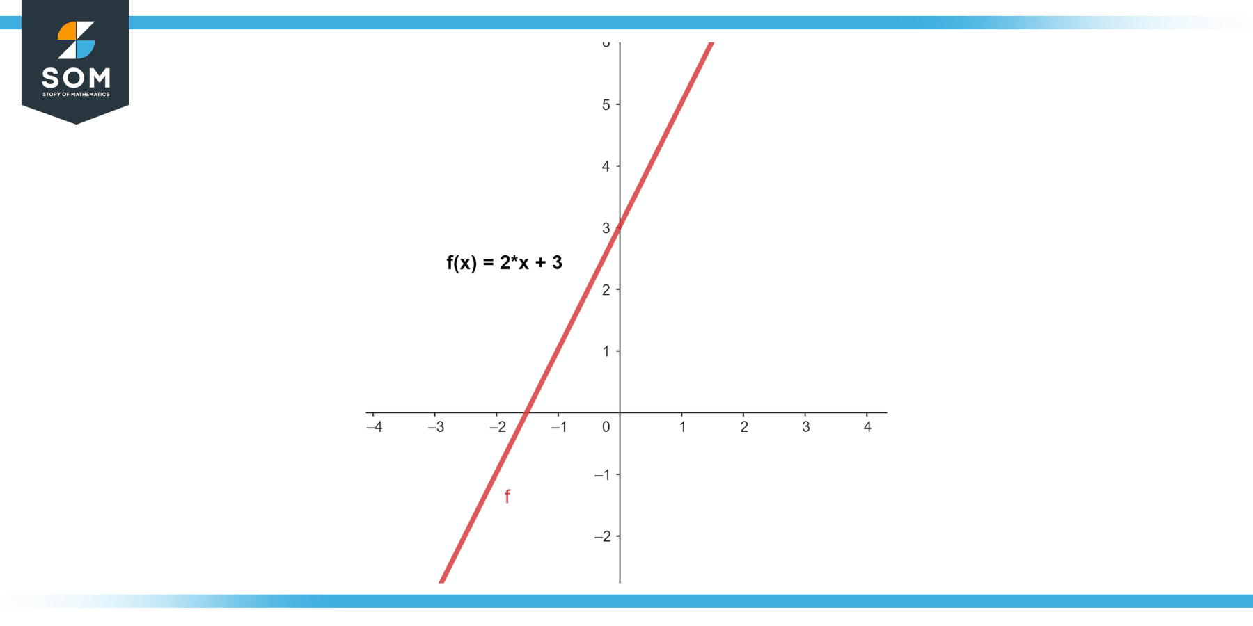
Figure-2.
Solution
The derivative of f(x) is:
f'(x) = 2
At x = 1, the slope of the tangent line is 2, so the slope of the normal line is the negative reciprocal, which is -1/2.
The y-coordinate of the point is:
f(1) = 2*1 + 3 = 5
so the point is (1, 5).
Using the point-slope form of a line, y – y1 = m(x – x1), where m is the slope and (x1, y1) is the point, the equation of the normal line is:
y – 5 = -1/2 (x – 1)
Example 2
Consider the function f(x) = x², and we want to find the normal line at the point where x = 1.
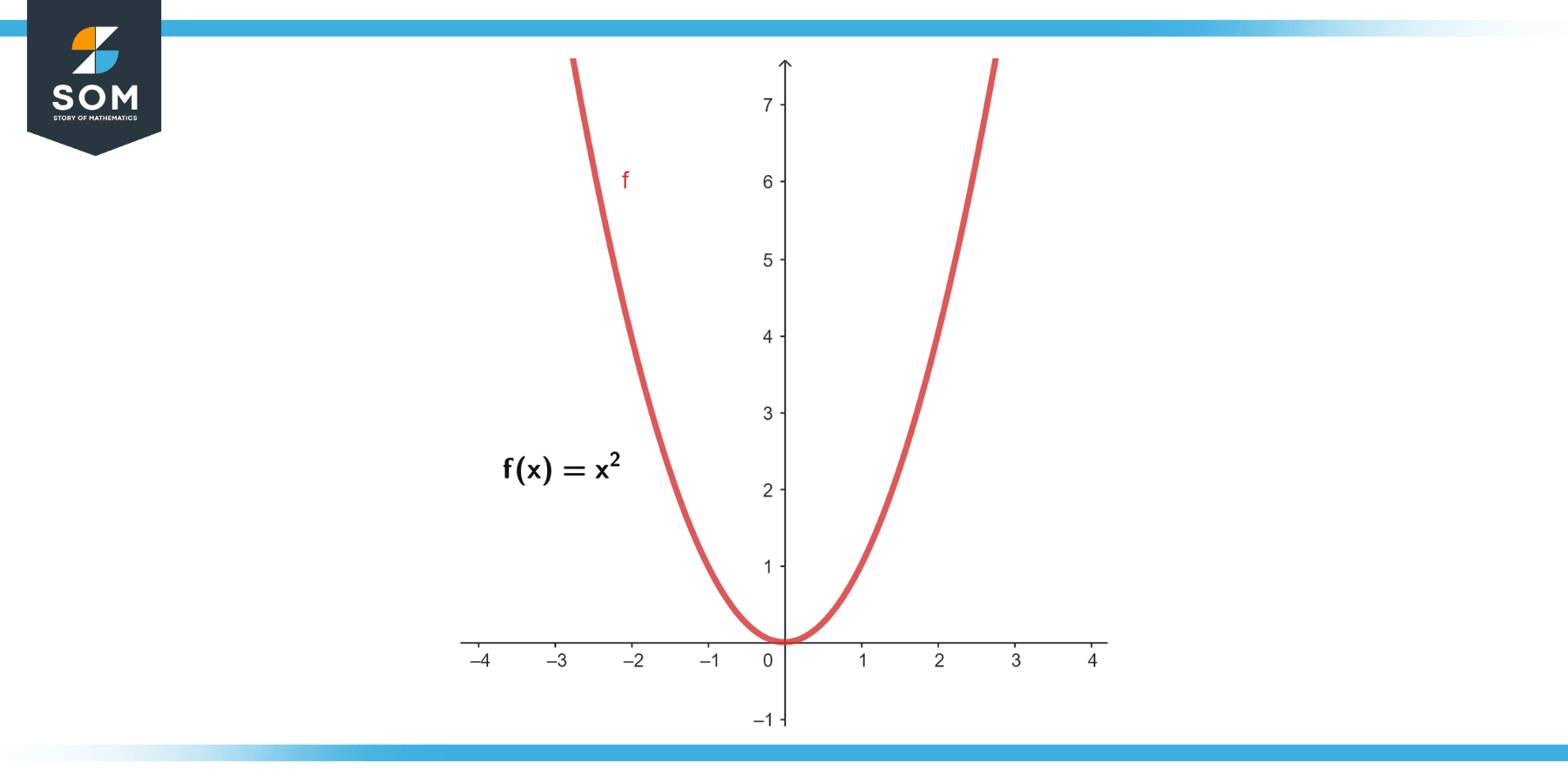
Figure-3.
Solution
The derivative of f(x) is:
f'(x) = 2x
At x = 1, the slope of the tangent line is 2, so the slope of the normal line is -1/2.
The y-coordinate of the point is:
f(1) = (1)²= 1
so the point is (1, 1).
The equation of the normal line is:
y – 1 = -1/2 (x – 1)
Example 3
Consider the function f(x) = x³, and we want to find the normal line at the point where x = 1.
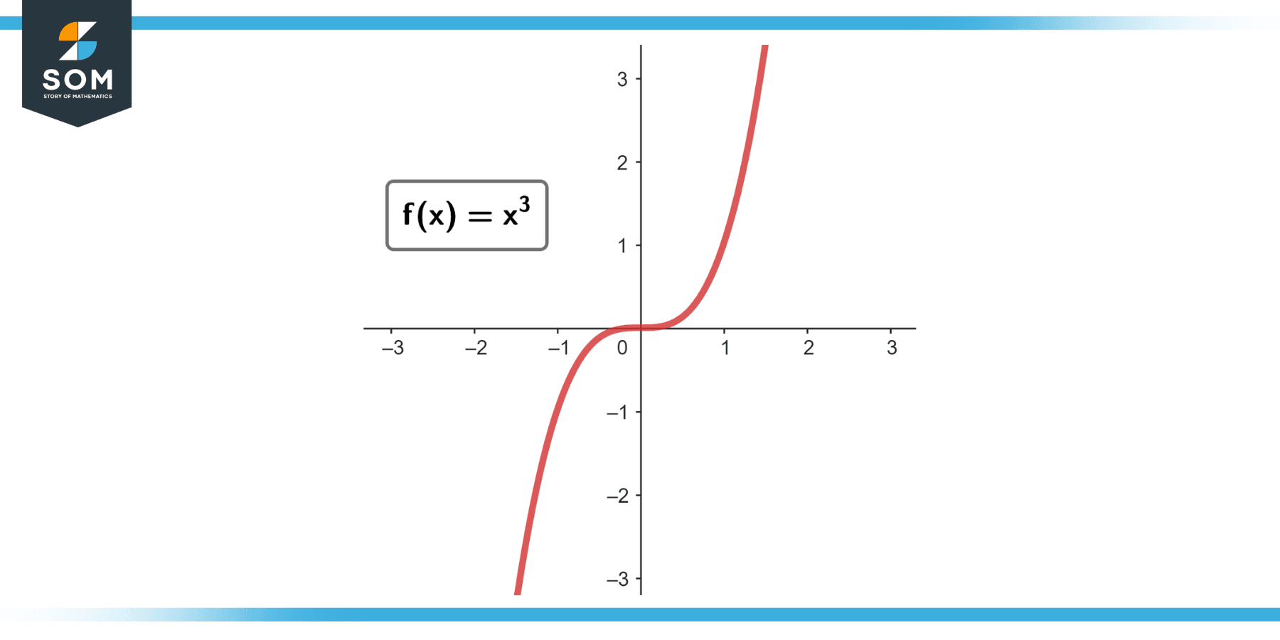
Figure-4.
Solution
The derivative of f(x) is:
f'(x) = 3x²
At x = 1, the slope of the tangent line is 3, so the slope of the normal line is -1/3.
The y-coordinate of the point is:
f(1) = (1)³= 1
so the point is (1, 1).
The equation of the normal line is:
y – 1 = -1/3 (x – 1)
Applications
Physics and Engineering
In physics, the concept of the normal line is crucial in understanding the laws of reflection and refraction. The incidence and reflection or refraction angles are measured relative to the normal line at the point of contact.
Geology and Geography
In geology, normal lines are used in understanding the structure and composition of different rock formations. Geographers use normal lines to understand and represent the Earth’s topography. Normal lines construct contour lines representing terrain on a 2D surface.
Robotics and Machine Vision
Normal lines are extensively used in robotics and machine vision. For instance, when a robot interacts with an object, knowing the normal line to the contact surface helps plan how to apply forces without slipping. In machine vision, normal maps add details to surfaces without increasing the complexity of the 3D model.
Aerospace Engineering
In aerodynamics, the pressure acting on an airplane wing or any aerodynamic surface is often decomposed into components along the tangent and the normal to the surface. This helps in calculating lift and drag forces.
Calculus
In multivariable calculus, the gradient of a function at a point gives a vector normal to the level surface of the function at that point. This is used in optimization problems, among other things.
All images were created with GeoGebra.