
This article explores the concept of the average rate of change over an interval, aiming to illuminate this mathematical tool in a manner accessible to everyone.
Defining Average Rate of Change Over an Interval
The average rate of change over an interval refers to the change in the value of a function between two points divided by the difference in the independent variables of these two points. In simpler terms, it measures how much the output (or dependent variable) changes per unit change in the input (or independent variable) over a specific interval.
Mathematically, it can be expressed as:
Average Rate of Change = [f(b) – f(a)] / (b – a)
where f(b) and f(a) are the function values at points b and a, respectively, and b and a are the endpoints of the interval on which the rate of change is being determined. This is essentially the slope of the secant line passing through the points (a, f(a)) and (b, f(b)) on the graph of the function.
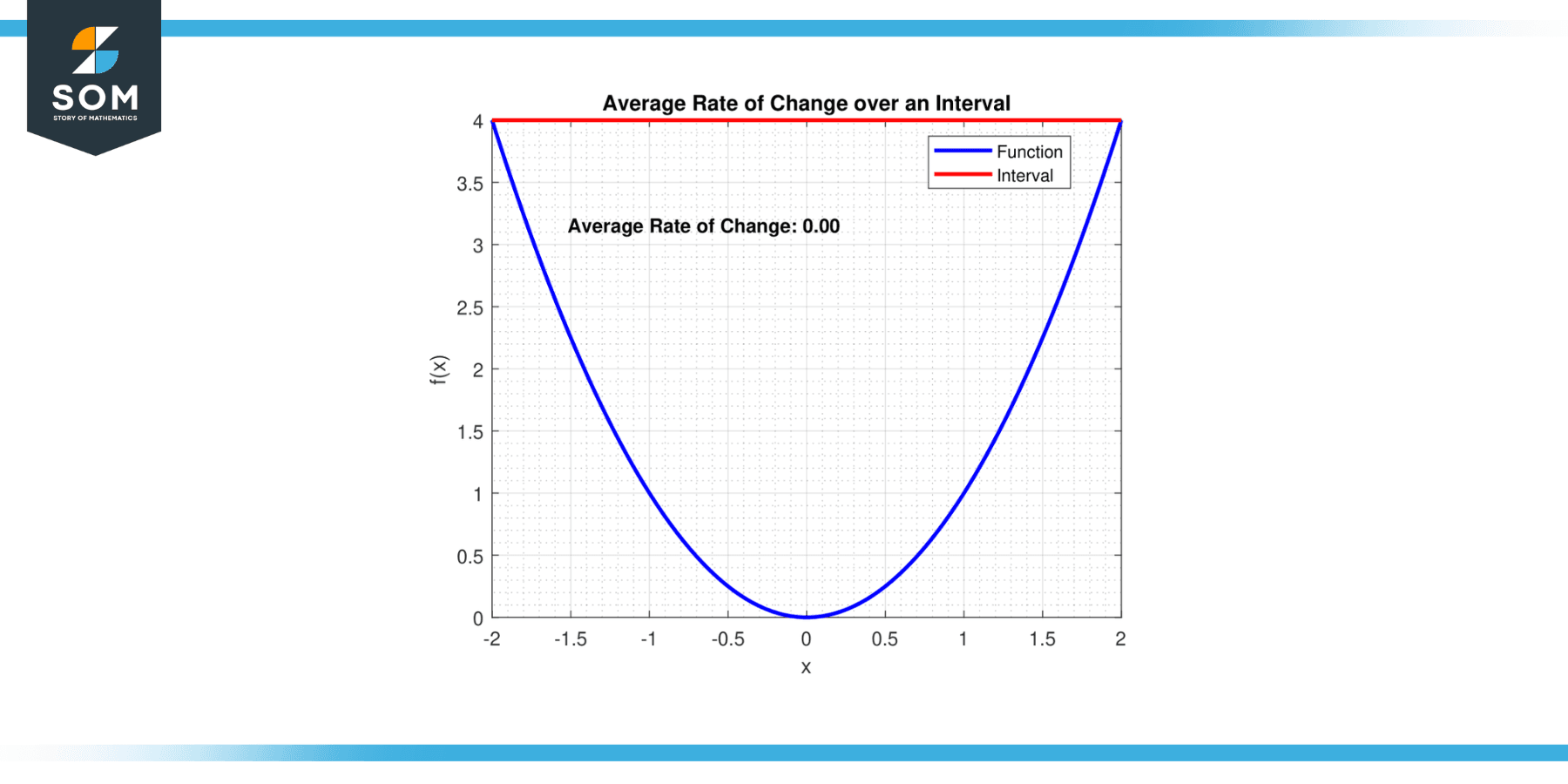
Figure-1.
The average rate of change is fundamental in calculus and underpins more complex ideas, such as the instantaneous rate of change and the derivative.
Properties
Much like many mathematical concepts, the average rate of change has certain properties integral to its understanding and application. These properties are fundamental aspects of the average rate of change behavior. Here are some of them in detail:
Linearity
One of the key properties of the average rate of change is its linearity, which stems from the fact that it represents the slope of the secant line between two points on a function graph. This essentially means that if the function being considered is linear (i.e., it represents a straight line), the average rate of change over any interval is constant and equals the slope of the line.
Dependence on Interval
The average rate of change is dependent on the specific interval chosen. In other words, the average rate of change between two different pairs of points (i.e., different intervals) on the same function can be different. This is particularly evident in non-linear functions, where the average rate of change is not constant.
Symmetry
The average rate of change is symmetric in that reversing the interval will only change the sign of the rate. If the average rate of change from ‘a’ to ‘b’ is calculated to be ‘r,’ then the average rate of change from ‘b’ to ‘a’ will be ‘-r.’
Interval Average vs. Instantaneous Change
The average rate of change over an interval gives an overall view of the behavior of a function within that interval. It does not reflect instantaneous changes within the interval, which may differ greatly. This fundamental concept leads to the idea of a derivative in calculus, which represents the instantaneous rate of change at a point.
Connection to Area Under Curve
In the context of integral calculus, the average rate of change of a function over an interval is equal to the average value of its derivative over that interval. This is a consequence of the fundamental theorem of calculus.
Exercise
Example 1
Linear Function Example
Given f(x) = 3x + 2. Find the average rate of change from x = 1 to x = 4.
Solution
Average Rate of Change = [f(4) – f(1)] / (4 – 1)
Average Rate of Change = [(34 + 2) – (31 + 2)] / (4 – 1)
Average Rate of Change = (14 – 5) / 3
Average Rate of Change = 3
This means that for every unit increase in x, the function increases by 3 units on average between x = 1 and x = 4.
Example 2
Quadratic Function Example
Suppose f(x) = x². Find the average rate of change from x = 2 to x = 5.
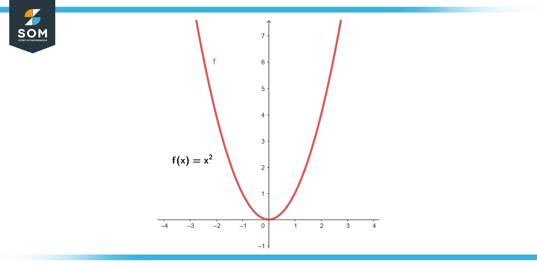
Figure-2.
Solution
Average Rate of Change = [f(5) – f(2)] / (5 – 2)
Average Rate of Change = [(5²) – (2²)] / (5 – 2)
Average Rate of Change = (25 – 4) / 3
Average Rate of Change = 7
Example 3
Exponential Function Example
Suppose f(x) = 2ˣ. Find the average rate of change from x = 1 to x = 3.
Average Rate of Change = [f(3) – f(1)] / (3 – 1)
Average Rate of Change = [(2³) – (2^1)] / (3 – 1)
Average Rate of Change = (8 – 2) / 2
Average Rate of Change = 3
Example 4
Cubic Function Example
Suppose f(x) = x³. Find the average rate of change from x = 1 to x = 2.
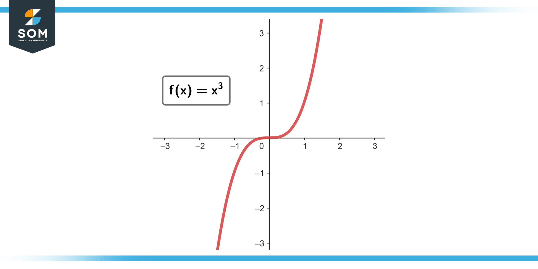
Figure-3.
Solution
Average Rate of Change = [f(2) – f(1)] / (2 – 1)
Average Rate of Change = [(2³) – (1³)] / (2 – 1)
Average Rate of Change = (8 – 1) / 1
Average Rate of Change = 7
Example 5
Square Root Function Example
Suppose f(x) = √x. Find the average rate of change from x = 4 to x = 9.
Solution
Average Rate of Change = [f(9) – f(4)] / (9 – 4)
Average Rate of Change = [(√9) – (√4)] / (9 – 4)
Average Rate of Change = (3 – 2) / 5
Average Rate of Change = 0.2
Example 6
Inverse Function Example
Suppose f(x) = 1/x. Find the average rate of change from x = 1 to x = 2.
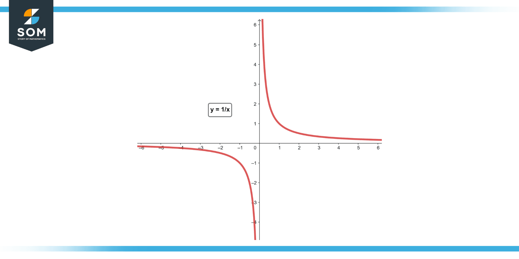
Figure-4.
Solution
Average Rate of Change = [f(2) – f(1)] / (2 – 1)
Average Rate of Change = [(1/2) – (1/1)] / (2 – 1)
Average Rate of Change = (-0.5) / 1
Average Rate of Change = -0.5
Example 7
Absolute Value Function Example
Suppose f(x) = |x|. Find the average rate of change from x = -2 to x = 2.
Solution
Average Rate of Change = [f(2) – f(-2)] / (2 – -2)
Average Rate of Change = [(2) – (2)] / (2 – -2)
Average Rate of Change = 0 / 4
Average Rate of Change = 0
Example 8
Trigonometric Function Example
Suppose f(x) = sin(x). Find the average rate of change from x = π/6 to x = π/3. (Note that we use radians for x in trigonometric functions.)
Solution
Average Rate of Change = [f(π/3) – f(π/6)] / (π/3 – π/6)
Average Rate of Change = [sin(π/3) – sin(π/6)] / (π/6)
Average Rate of Change = [(√3/2) – (1/2)] / (π/6)
Average Rate of Change = (√3 – 1) / (π/2)
Average Rate of Change ≈ 0.577
Applications
The average rate of change over an interval is widely applicable in various fields. Here are a few examples:
Physics
In physics, the average rate of change is commonly used in kinematics, the study of motion. For example, the average velocity of an object over a given time interval is the average rate of change of its position with respect to time during that interval. Similarly, the average acceleration is the average rate of change of velocity.
Economics
In economics and finance, the average rate of change can be used to understand changes in various metrics over time. For instance, it can be used to analyze the average growth rate of a company’s revenue or profits over several years. It could also be used to evaluate changes in stock prices, GDP, unemployment rates, etc.
Biology
In population biology and ecology, the average rate of change can be used to measure the growth rate of a population. This could be the rate of change of the number of individuals in a population or the change in the concentration of a substance in an ecosystem.
Chemistry
In chemistry, the rate of reaction is essentially an average rate of change—it represents the change in concentration of a reactant or product per unit of time.
Environment Science
In environmental studies, the average rate of change can be used to measure pollution levels, temperature changes (global warming), deforestation rates, and many more.
Medical Science
In medical science, it can measure the rate of change in a patient’s condition over time. This could be the change in heart rate, blood sugar levels, or tumor growth rate.
Geography
In geography, it’s used to assess changes in various parameters over time, such as the erosion rate of a riverbank, glacier melting rates, or even urban sprawl rates.
Computer Science
In computer science, the average rate of change can be used in algorithms to predict future trends based on past data.
These are just a few examples. The average rate of change is an essential mathematical tool that finds wide-ranging applications across virtually all fields of science, technology, and beyond.
All images were created with GeoGebra and MATLAB.