JUMP TO TOPIC
The magic of mathematics unfolds as we delve into the fascinating world of direct variation equations. Often encountered in academic and real-world situations, this equation paints a vivid picture of relationships where one variable changes directly from another.
It helps us explain phenomena like the speed of a car relating to the time it takes to reach a destination or how the cost of goods changes with quantity. The mathematical simplicity of direct variation belies its profound implications, giving us a glimpse into the predictable and proportional relationships that govern our world.
Dive into this article to unravel the mystery, utility, and beauty of direct variation equations and understand how they shape our understanding of the world.
Definition of Direct Variation Equation
A direct variation equation is a mathematical relationship between two variables where the ratio of the two remains constant. In other words, when one variable increases, the other increases proportionally, and vice versa.
This relationship is often expressed in the form y = kx, where y and x are the two variables, and k is the constant of variation. If you know the value of one variable, you can use the direct variation equation to find the value of the other variable.
The constant k is determined by the specific relationship between the two variables. Direct variation equations play a vital role in understanding various real-world scenarios, from physics to economics, allowing for predictable and consistent calculations and predictions.
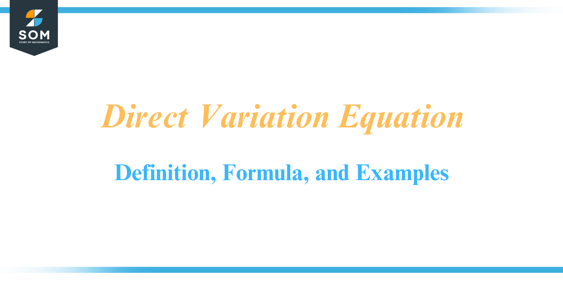
Below is the figure-1, we present a generic representation of the direct variation equations.
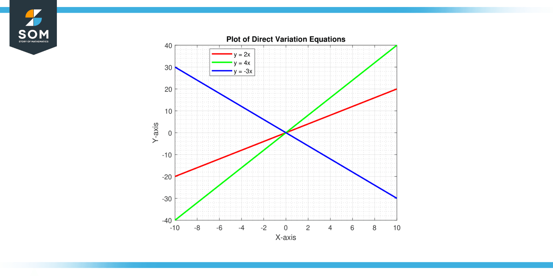
Figure-1.
Historical Significance
The concept of direct variation, also known as direct proportion, has roots in ancient mathematics. The principle of direct variation underpins the concept of ratio and proportion, which were pivotal in the mathematical systems of ancient civilizations.
Ancient Babylonians (c. 1800 BCE)
Babylonian mathematics used ratios extensively, though their understanding of proportion didn’t exactly equate to our modern concept of direct variation. They used ratios to solve problems related to trade, land measurement, and geometric calculations.
Ancient Greeks (c. 300 BCE)
In his work “Elements,” Greek mathematician Euclid formalized the concept of ratios and proportions. His definition of equal ratios can be seen as an early exploration of direct variation.
Middle Ages and Renaissance
During this period, European mathematicians translated Greek and Arabic mathematical texts and incorporated their knowledge, further developing concepts of ratios and proportions.
17th Century
With the advent of analytical geometry and calculus by mathematicians like René Descartes and Isaac Newton, the concept of direct variation became clearer. Descartes introduced the concept of representing equations graphically, which led to the understanding that direct variation equations represent straight lines passing through the origin.
19th Century Onwards
As mathematics became more abstract, the concept of functions was formalized. The direct variation was then seen as a specific type of function – a linear function with a y-intercept of 0.
The concept of direct variation has been refined and abstracted over millennia, playing a fundamental role in our understanding of the mathematical world. It’s crucial in various fields such as physics, economics, biology, and engineering, demonstrating the power of this relatively simple mathematical relationship.
Properties
The properties of the direct variation equation are:
Constant Ratio
In a direct variation, the ratio of the two variables is always constant. This means that for any two pairs of corresponding values of ‘x’ and ‘y’ (x1, y1) and (x2, y2), the ratio y1/x1 equals y2/x2.
Origin Passage
A direct variation equation always passes through the origin (0,0) in a graph. This is because when one variable is zero, the other is also zero. Therefore, the graph of a direct variation is a straight line passing through the origin.
Proportional Change
The variables in a direct variation change proportionally. If ‘x’ doubles, ‘y’ doubles; if ‘x’ triples, ‘y’ triples, and so on. Similarly, if ‘x’ is halved, ‘y’ is also halved. This is because of the constant ratio (k) between ‘x’ and ‘y’.
Nonzero Constant
The variation ‘k’ constant is never zero in a direct variation. If ‘k’ were zero, the equation would be y = 0, which does not represent a variable relationship.
Unit Rate
The constant of variation ‘k’ can also be considered as the unit rate or slope of the line in the coordinate plane. It represents the amount by which ‘y’ changes for every unit change in ‘x’.
Inverse Relationship With Reciprocal
While in a direct variation, y varies directly as x, in its reciprocal form, x varies directly as 1/y. This relationship solves many problems where the direct variation relationship is known, but the inverse relationship is required.
Applications
Direct variation equations are used in various disciplines to describe relationships where changes in one quantity lead to proportional changes in another. Here are some examples:
Physics and Engineering
Direct variation is fundamental to many laws of physics and principles of engineering. For instance, Ohm’s Law states that the current through a conductor between two points is directly proportional to the voltage across the two points. Here, the constant of proportionality is the resistance.
Chemistry
In gas laws, the volume of a gas varies directly with its temperature when pressure and the amount of gas are kept constant (Charles’s Law). Also, the pressure of a gas varies directly with its temperature when the volume and the amount of gas are kept constant (Gay-Lussac’s Law).
Economics
Direct variation equations are used in economics to describe the relationship between supply and demand, the effect of interest rates on investment, the cost of goods based on quantity, and much more. For example, the total cost of manufacturing ‘n’ items is usually a direct variation of ‘n’.
Biology
In biology, direct variation can explain phenomena like the relationship between the metabolic rate of an organism and its body mass.
Computer Science
In computer science, direct variation describes algorithm complexity in Big O notation. For example, in an O(n) algorithm, the time it takes to execute it varies directly with the input data size.
Astronomy
Kepler’s Third Law states that the square of the period of revolution of a planet around the sun is directly proportional to the cube of its average distance from the sun.
Exercise
Example 1
If y varies directly as x, and y = 20 when x = 5, find the variation (k) constant and write the variation equation.
Solution
From the equation y = kx, we can solve for k as:
y/x = k
When y = 20 and x = 5, we find:
k = 20/5
k = 4
So, the equation of variation is y = 4 * x.
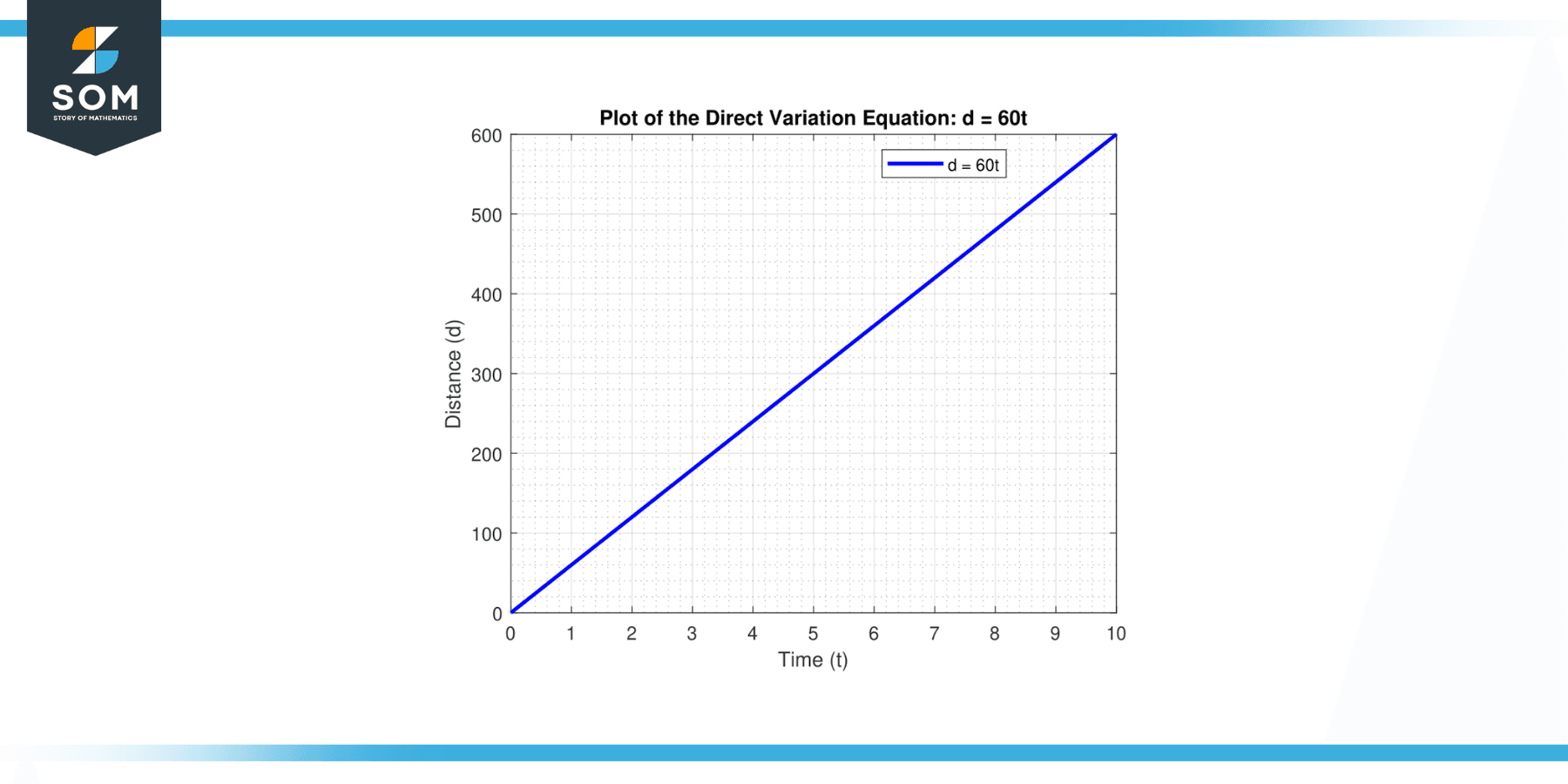
Figure-2.
Example 2
The weight of an object varies directly with its volume. If an object with a volume of 3 cubic meters weighs 6 kg, how much would an object with a volume of 7 cubic meters weigh?
Solution
The equation for this direct variation is:
Weight = k * Volume
When volume = 3, we get:
weight = 6
and
k = 6 / 3
k = 2
Therefore, the weight of an object with a volume of 7 cubic meters would be 2 * 7 = 14 kg.
Example 3
The amount of money (M) you earn varies directly with the number of hours (h) you work. If you earn $150 for 10 hours of work, what is the equation of variation?
Solution
Here, M = k * h. Since M = $150 when h = 10, we get:
k = 150 / 10
k = 15
So, the equation of variation is M = 15 h.
Example 4
Using the previous example, how much money would you earn for 15 work hours?
Solution
With the equation M = 15 h, you would earn:
M = 15 * 15
M = $225 for 15 hours of work
Example 5
The force of gravity acting on an object is directly proportional to its mass. If an object with a mass of 2 kg has a gravitational force of 19.6 N, what would be the gravitational force acting on an object of mass 5 kg?
Solution
The equation for this direct variation is:
F = k * m
With F = 19.6 N when m = 2 kg, we find:
k = 19.6 / 2
k = 9.8
So, the gravitational force on an object of mass 5 kg would be 9.8 * 5 = 49 N.
Example 6
The cost of apples (C) varies directly with the number of apples bought (n). If 4 apples cost $8, how much would 10 apples cost?
Solution
In this direct variation:
C = k * n
When n = 4, C = $8, we get:
k = 8 / 4
k = 2
Therefore, the cost of 10 apples would be 2 * 10 = $20.
Example 7
The distance (d) a car travels varies directly with the time (t) it travels. If a car travels 300 km in 5 hours, what is the equation of variation?
Solution
Here, d = k * t. Since d = 300 km when t = 5 hours, we get
k = 300 / 5
k = 60
Therefore, the equation of variation is d = 60 t.
Figure-3.
Example 8
Using the previous example, how far would the car travel in 8 hours?
Solution
Using the equation d = 60 t, the car would travel:
d = 60 * 8
d = 480 km in 8 hours
All images were created with MATLAB.