
Euler’s Method is a cornerstone in numerical approximation, offering a simple yet powerful approach to solving differential equations.
Named after the esteemed mathematician Leonhard Euler, this technique has revolutionized scientific and engineering disciplines by enabling researchers and practitioners to tackle complex mathematical problems that defy analytical solutions.
Euler’s Method allows for approximating solutions to differential equations by breaking them down into smaller, manageable steps. This article delves into the intricacies of Euler’s Method by highlighting the crucial interplay between numerical computation and the fundamental concepts of calculus.
We journeyed to uncover its underlying principles, understand its strengths and limitations, and explore its diverse applications across various scientific domains.
Definition of Euler’s Method
Euler’s Method is a numerical approximation technique used to numerically solve ordinary differential equations (ODEs). It is named after the Swiss mathematician Leonhard Euler, who made significant contributions to the field of mathematics.
The method provides an iterative approach to estimating the solution of an initial value problem by breaking the continuous differential equation into discrete steps. Euler’s Method advances from one point to the next by approximating the derivative at each step, gradually constructing an approximate solution curve.
The method is based on the concept of the tangent line to an ODE at a given point and employs simple calculations to estimate the next point on the solution trajectory. Below we present a generic representation of Euler’s method approximation in figure-1.
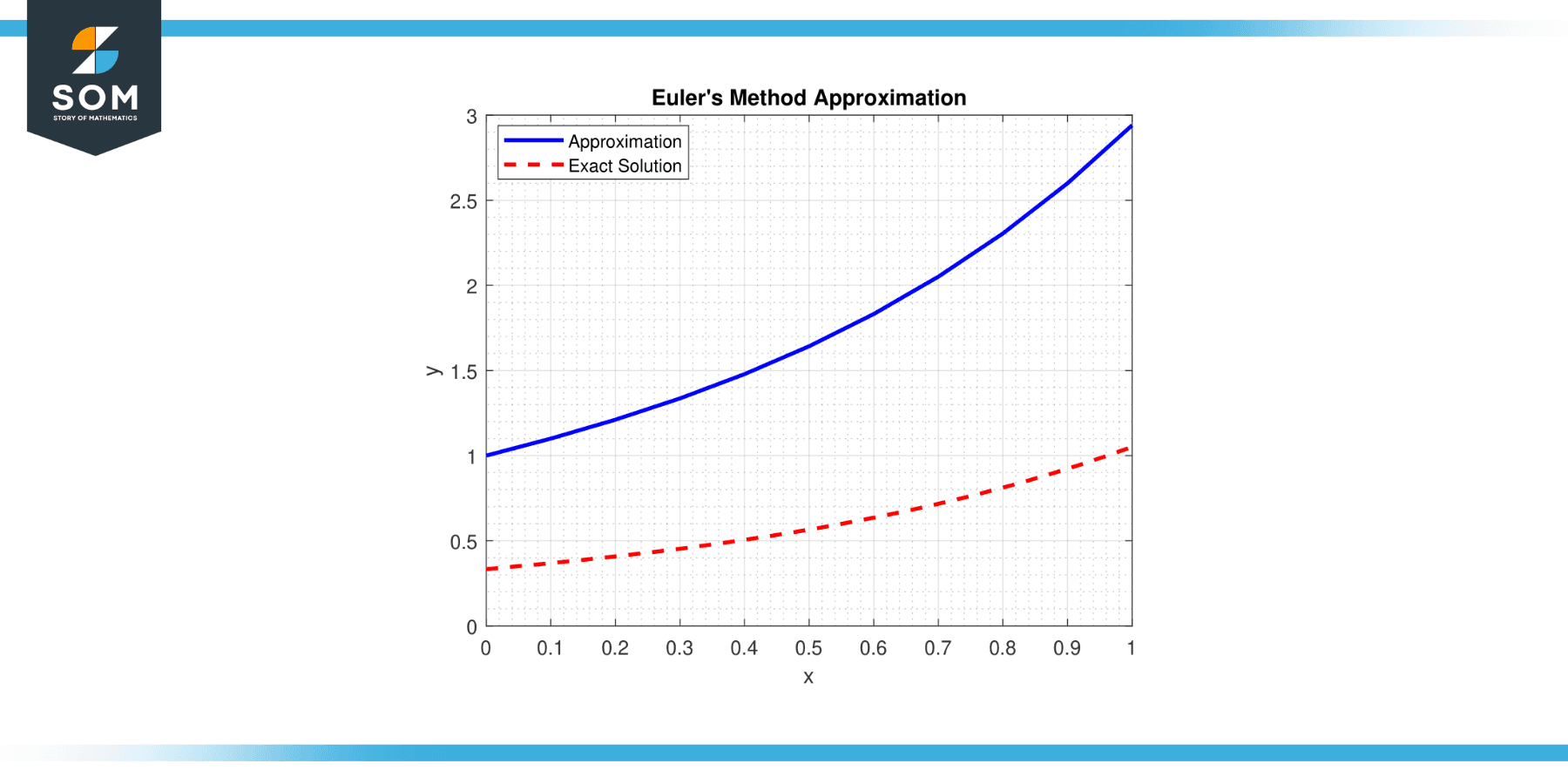
Figure-1.
Although Euler’s Method is relatively straightforward, it is a foundation for more advanced numerical techniques and has immense practical significance in various scientific and engineering fields where analytic solutions may be challenging or impossible to obtain.
Evaluating Euler’s Method
Evaluating Euler’s Method involves following a systematic process to approximate the solution of an ordinary differential equation (ODE). Here is a step-by-step description of the process:
Formulate the ODE
Start by having a given ODE in the form dy/dx = f(x, y), along with an initial condition specifying the value of y at a given x-value (e.g., y(x₀) = y₀).
Choose the Step Size
Determine the desired step size (h) to divide the interval of interest into smaller intervals. A smaller step size generally yields more accurate results but increases computational effort.
Set up the Discretization
Define a sequence of x-values starting from the initial x₀ and incrementing by the step size h: x₀, x₁ = x₀ + h, x₂ = x₁ + h, and so on, until the desired endpoint is reached.
Initialize the Solution
Set the initial solution value to the given initial condition: y(x₀) = y₀.
Repeat the Iteration
Continue iterating the method by moving to the next x-value in the sequence and updating the solution using the computed derivative and step size. Repeat this process until reaching the desired endpoint.
Output the Solution
Once the iteration is complete, the final set of (x, y) pairs represents the numerical approximation of the solution to the ODE within the specified interval.
Iterate the Method
For each xᵢ in the sequence of x-values (from x₀ to the endpoint), apply the following steps:
- Evaluate the derivative: Compute the derivative f(x, y) at the current xᵢ and y-value.
- Update the solution: Multiply the derivative by the step size h and add the result to the previous solution value. This yields the next approximation of the solution: yᵢ₊₁ = yᵢ + h * f(xᵢ, yᵢ).
It is important to note that Euler’s Method provides an approximate solution, and the accuracy depends on the chosen step size. Smaller step sizes generally yield more accurate results but require more computational effort. Higher-order methods may be more appropriate for complex or highly curved solution curves to minimize the accumulated error.
Properties
Approximation of Solutions
Euler’s Method provides a numerical approximation of the solution to an ordinary differential equation (ODE). It breaks down the continuous ODE into discrete steps, allowing for the estimation of the solution at specific points.
Local Linearity Assumption
The method assumes that the behavior of the solution between two adjacent points can be approximated by a straight line based on the slope at the current point. This assumption holds for small step sizes, where a tangent line can closely approximate the solution curve.
Discretization
The method employs a step size (h) to divide the interval over which the solution is sought into smaller intervals. This discretization allows for evaluating the derivative at each step and the progression toward the next point on the solution curve.
Global Error Accumulation
Euler’s Method is prone to accumulating errors over many steps. This cumulative error arises from the linear approximation employed at each step and can lead to a significant deviation from the true solution. Smaller step sizes generally reduce the overall error.
Iterative Process
Euler’s Method is an iterative process where the solution at each step is determined based on the previous step’s solution and the derivative at that point. It builds the approximation by successively calculating the next point on the solution trajectory.
Algorithm
Euler’s Method follows a simple algorithm for each step: (a) Evaluate the derivative at the current point, (b) Multiply the derivative by the step size, (c) Update the solution by adding the product to the current solution, (d) Move to the next point by increasing the independent variable by the step size.
First-Order Approximation
Euler’s Method is a first-order numerical method, meaning its local truncation error is proportional to the square of the step size (O(h^2)). Consequently, it may introduce significant errors for large step sizes or when the solution curve is highly curved.
Versatility and Efficiency
Despite its limitations, Euler’s Method is widely used for its simplicity and efficiency in solving initial value problems. It serves as the foundation for more sophisticated numerical methods, and its basic principles are extended and refined in higher-order methods like the Improved Euler Method and Runge-Kutta methods.
Understanding the properties of Euler’s Method helps to appreciate its strengths and limitations, aiding in selecting appropriate numerical methods based on the specific characteristics of the problem.
Applications
Despite its simplicity, Euler’s method finds applications in various fields where numerical approximation of ordinary differential equations (ODEs) is required. Here are some notable applications of Euler’s Method in different fields:
Physics
Euler’s Method is extensively used in physics for simulating the motion of objects under the influence of forces. It allows for the numerical solution of ODEs arising from physical laws such as Newton’s laws of motion or thermodynamics. Applications range from simple projectile motion to complex celestial bodies or fluid dynamics simulations.
Engineering
Euler’s Method plays a vital role in modeling and analyzing dynamic systems. It enables the numerical solution of ODEs that describe the behavior of systems such as electrical circuits, control systems, mechanical structures, and fluid flow. Using Euler’s Method, engineers can understand and predict system responses without relying solely on analytical solutions.
Computer Science
Euler’s Method forms the foundation for many numerical algorithms used in computer science. It is crucial for solving differential equations that arise in areas like computer graphics, simulation, and optimization. Euler’s Method is employed to model physical phenomena, simulate particle dynamics, solve differential equations in numerical analysis, and optimize algorithms through iterative processes.
Biology and Medicine
In biological and medical sciences, Euler’s Method models biological processes, such as population growth, pharmacokinetics, and drug-dose response relationships. It allows researchers to investigate the dynamics of biological systems and simulate the effects of interventions or treatment strategies.
Economics and Finance
Euler’s Method is utilized in economic and financial modeling to simulate and analyze economic systems and financial markets. It enables the numerical solution of economic equations, asset pricing models, portfolio optimization, and risk management. Euler’s Method facilitates the study of complex economic dynamics and the assessment of economic policies and investment strategies.
Environmental Science
Environmental scientists utilize Euler’s Method to model ecological systems and analyze the dynamics of environmental processes. It enables the simulation of population dynamics, ecosystem interactions, climate modeling, and pollutant dispersion. Euler’s Method aids in predicting the effects of environmental changes and understanding the long-term behavior of ecosystems.
Astrophysics and Cosmology
Euler’s Method is employed in astrophysics and cosmology to model the evolution and behavior of celestial objects and the universe. It helps study the dynamics of planetary orbits, stellar evolution, galaxy formation, and cosmological phenomena. Euler’s Method allows researchers to simulate and analyze complex astronomical systems and investigate the universe’s origins.
Euler’s Method is a versatile and foundational tool in numerous fields, providing a practical approach to numerically solve ODEs and gain insights into dynamic systems lacking analytical solutions. Its applications span scientific research, engineering design, computational modeling, and decision-making processes.
Exercise
Example 1
Approximating a First-Order Differential Equation
Consider the differential equation dy/dx = x^2 with the initial condition y(0) = 1. Use Euler’s Method with a step size of h = 0.1 to approximate the solution at x = 0.5.
Solution
Using Euler’s Method, we start with the initial condition y(0) = 1 and iteratively calculate the next approximation using the formula:
y_i+1 = y_i + h * f(x_i, y_i)
where f(x, y) represents the derivative.
Step 1: At x = 0, y = 1.
Step 2: At x = 0.1, y = 1 + 0.1 * (0^2) = 1.
Step 3: At x = 0.2, y = 1 + 0.1 * (0.1^2) = 1.001.
Step 4: At x = 0.3, y = 1 + 0.1 * (0.2^2) = 1.004.
Step 5: At x = 0.4, y = 1 + 0.1 * (0.3^2) = 1.009.
Step 6: At x = 0.5, y = 1 + 0.1 * (0.4^2) = 1.016.
Therefore, the approximation of the solution at x = 0.5 is y ≈ 1.016.
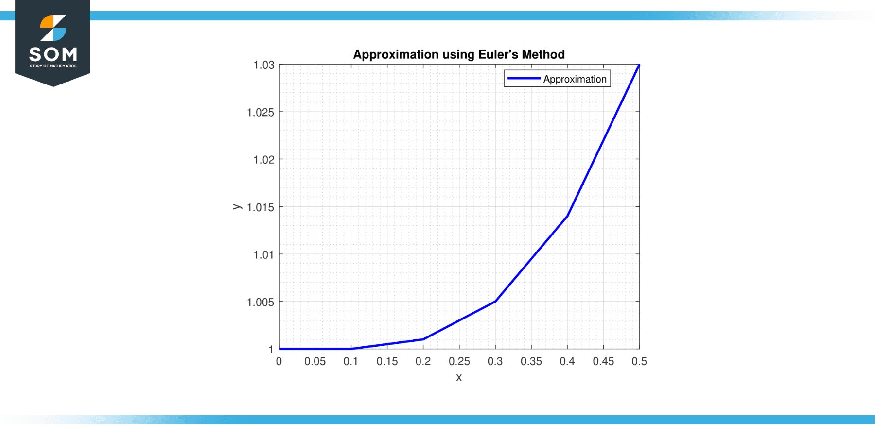
Figure-2.
Example 2
Approximating a Second-Order Differential Equation
Consider the differential equation d^2y/dx^2 + 2dy/dx + 2y = 0 with initial conditions y(0) = 1 and dy/dx(0) = 0. Use Euler’s Method with a step size of h = 0.1 to approximate the solution at x = 0.4.
Solution
We convert the second-order equation into a system of first-order equations to approximate the solution using Euler’s Method.
Let u = dy/dx. Then, the given equation becomes a system of two equations:
du/dx = -2u – 2y
and
dy/dx = u
Using Euler’s Method with a step size of h = 0.1, we approximate the values of u and y at each step.
Step 1: At x = 0, y = 1 and u = 0.
Step 2: At x = 0.1, y = 1 + 0.1 * (0) = 1 and u = 0 + 0.1 * (-2 * 0 – 2 * 1) = -0.2.
Step 3: At x = 0.2, y = 1 + 0.1 * (-0.2) = 0.98 and u = -0.2 + 0.1 * (-2 * (-0.2) – 2 * 0.98) = -0.242.
Step 4: At x = 0.3, y = 0.98 + 0.1 * (-0.242) = 0.9558 and u = -0.242 + 0.1 * (-2 * (-0.242) – 2 * 0.9558) = -0.28514.
Step 5: At x = 0.4, y = 0.9558 + 0.1 * (-0.28514) = 0.92729 and u = -0.28514 + 0.1 * (-2 * (-0.28514) – 2 * 0.92729) = -0.32936.
Therefore, the approximation of the so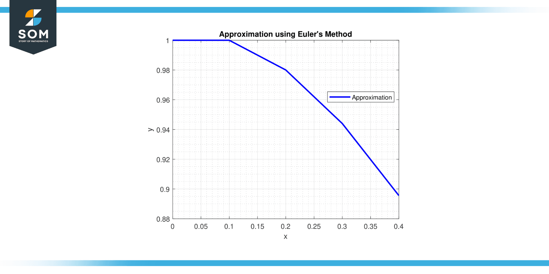 lution at x = 0.4 is y ≈ 0.92729.
Figure-3.
Example 3
Approximating a System of Differential Equations
Consider the differential equations dx/dt = t – x and dy/dt = x – y with initial conditions x(0) = 1 and y(0) = 2. Use Euler’s Method with a step size of h = 0.1 to approximate x and y values at t = 0.5.
Solution
Using Euler’s Method, we approximate the values of x and y at each step using the given system of differential equations.
Step 1: At t = 0, x = 1 and y = 2.
Step 2: At t = 0.1, x = 1 + 0.1 * (0 – 1) = 0.9 and y = 2 + 0.1 * (1 – 2) = 1.9.
Step 3: At t = 0.2, x = 0.9 + 0.1 * (0.1 – 0.9) = 0.89 and y = 1.9 + 0.1 * (0.9 – 1.9) = 1.89.
Step 4: At t = 0.3, x = 0.89 + 0.1 * (0.2 – 0.89) = 0.878 and y = 1.89 + 0.1 * (0.89 – 1.89) = 1.88.
Step 5: At t = 0.4, x = 0.878 + 0.1 * (0.3 – 0.878) = 0.8642 and y = 1.88 + 0.1 * (0.878 – 1.88) = 1.8692.
Step 6: At t = 0.5, x = 0.8642 + 0.1 * (0.4 – 0.8642) = 0.84758 and y = 1.8692 + 0.1 * (0.8642 – 1.8692) = 1.86038.
Therefore, the approximation of the x and y values at t = 0.5 is x ≈ 0.84758 and y ≈ 1.86038.
All images were created with MATLAB.