 To graph a function ( f(x) ), I always begin by determining its domain and range. The domain of a function represents all the possible input values ( x ) can take, while the range is the set of all possible output values ( f(x) ) can produce.
Identifying these elements helps me understand the function’s behavior and where on the graph it will be defined.
For a continuous function, I then draw a line or curve through these points, extending to the edges of the domain and within the confines of the range. These steps construct an accurate graph that visually represents the function’s behavior.
Stay with me as I reveal how this visual tool unlocks a deeper comprehension of mathematical relationships, charting a course through the world of algebraic expressions and equations.
Steps for Graphing a Function
Graphing a function can seem daunting, but I’ll walk you through the process with some easy steps. Remember, a function is a relation where each input corresponds to exactly one output.

Determine the Domain and Range: The domain of a function is the set of all possible input values (usually x), while the range is the set of possible output values (usually y). These are the real numbers for which the function is defined.
Set Up a Table of Values: Start by choosing a set of input values from the domain. Then, calculate the corresponding output values to get ordered pairs.
Input (x) Output (f(x)) -2 f(-2) = … -1 f(-1) = … 0 f(0) = … 1 f(1) = … 2 f(2) = … Plot the Ordered Pairs: On the graph paper, mark each ordered pair as a point. The x-coordinate represents the input, and the y-coordinate the output value.
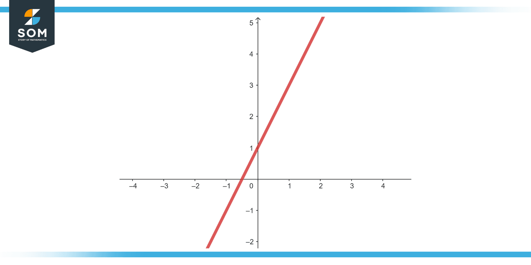
Draw the Curve or Line: Connect the points smoothly. If it is a straight line, ensure you’ve plotted at least two points, one being the y-intercept ( (0, b) ) where the graph crosses the y-axis, and calculate the slope as the rise over run $\frac{\Delta y}{\Delta x}$.
Test for Function with Vertical Line Test: To verify if a graph represents a function, use the vertical line test. Draw vertical lines across the graph. If any vertical line crosses the graph at more than one point, then it’s not a function.
Remember, the slope determines how steep the line is, and the y-intercept gives you a starting point on the graph. For more complex functions, you might need to calculate additional points or use other methods like transformations. Keep practicing and soon plotting any function will feel like a breeze!
Advanced Techniques in Graphing
When I graph a function $$ f(x) $$, I first consider its derivative to understand the slope and behavior of the curve. If the derivative, $$ f'(x) $$, is positive, the function is increasing, and if it’s negative, the function is decreasing.
The slope of the tangent to the curve at any point is the value of the derivative at that point. For instance, a square root function like $$ f(x) = \sqrt{x} $$ has a derivative of $$ f'(x) = \frac{1}{2\sqrt{x}} $$. Observing this derivative, I can see that the slope is positive but decreases as x increases.
Identifying the intercepts is also essential. The y-intercept is found when x=0, which is merely $$ f(0) $$. To find the x-intercepts, I solve for when $$ f(x) = 0 $$.
For the square root function, $$ \sqrt{x} = 0 $$ only when x=0, indicating that the graph touches the origin.
For advanced graphing, I make use of asymptotes. Vertical asymptotes occur at values of x where the function is undefined, and horizontal asymptotes indicate the value that the function approaches as x goes to infinity.
For example, the function $$ f(x) = \frac{1}{x} $$ has a vertical asymptote at x=0 and a horizontal asymptote at y=0.
Technology like graphing calculators and graphing apps can be helpful. Many web resources are available, some offering a free trial period, allowing me to explore different graphing tools. Here’s a simple table summarizing the relationships between various function characteristics and the graph’s appearance:
| Characteristic | Implication on Graph |
|---|---|
| Positive slope | Upward trend |
| Negative slope | Downward trend |
| Y-intercept | Spot where the graph crosses the y-axis |
| X-intercept | Spot(s) where the graph crosses the x-axis |
| Vertical asymptote | Value(s) x cannot take |
| Horizontal asymptote | Value y approaches at infinity |
Professional fields, especially in science and engineering, often necessitate graphing complex functions.
When working with these, additional attention to the equation helps in identifying key features like symmetry, periodicity, and other behaviors indicative of more complex curves and charts. Remember, a graph reveals a multitude of characteristics about a function that might not be immediately evident from the equation alone.
Conclusion
In our walkthrough, we’ve explored the fundamentals needed to graph a function, ( f(x) ), efficiently and accurately.
Remember, the journey begins by pinpointing the critical points and identifying any asymptotes that might inform the shape of our graph.
My next step is always to locate the function’s points by inputting values for ( x ) and finding the corresponding ( f(x) ) values. This step is crucial; it grounds my graph in concrete coordinates and starts to give me a feel for the function’s behavior.
Next, I join these points with either a line or curve, extending it according to the function’s defined behavior over its domain.
Drawing tangent lines is sometimes necessary when dealing with derivative graphs, such as when ( f'(x) ) expresses the slope at any given point on the original function’s graph.
Let’s not forget to apply the vertical line test for functions to ensure our graph represents a function properly. A vertical line intersecting the graph at more than one point would show a violation of the function definition, indicating that every input must map to exactly one output.
If you’ve followed these steps, you’ve done more than just sketch lines and curves; you’ve created a visual representation that encapsulates the essence of a mathematical function.
Whether simple linear functions or more complex polynomial ones, the graphing principles remain the same.
I encourage revisiting these steps whenever you’re graphing a function, and with practice, the process will become second nature.
As you continue to chart these mathematical territories, may your graphs always be accurate reflections of the functions they represent.