JUMP TO TOPIC
To graph a function, I begin by determining the domain and range, which are the set of all possible inputs (x-values) and outputs (y-values) respectively.
With this foundation, I plot points on the coordinate plane where each point represents an $(x, y)$ pair that satisfies the function’s equation.
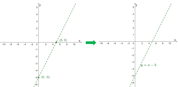
For example, if I’m working with a simple linear function like $y = mx + b$, where $m$ is the slope and $b$ is the y-intercept, I locate the intercept on the y-axis and use the slope to find other points, drawing a straight line through them.
Functions can be more complex, such as quadratic equations of the form $y = ax^2 + bx + c$, which create parabolic graphs. I plot their vertex, the highest or lowest point of the parabola, by using the formula $(-\frac{b}{2a}, f(-\frac{b}{2a}))$ and then sketch the curve through this point.
Graphing functions allow me to visually interpret mathematical relationships and patterns, making it a crucial skill in both academic and real-world applications. Stick around to discover the intriguing connections between a function’s algebraic expression and its graphical counterpart.
Exploring the Basics of Functions
When I start to graph a function, I like to remember that a function, in mathematics, is essentially a relationship that pairs each input with exactly one output. Inputs and outputs here are typically real numbers. I’ll give you a rundown of some critical terms:
- Input: This is the value we give to a function, commonly represented by the variable $x$.
- Output: The value that comes out from the function after we input $x$, often denoted as $f(x)$.
- Domain: All the possible inputs a function can accept.
- Range: All the possible outputs a function can produce.
| Term | Symbol | Description |
|---|---|---|
| Input | $x$ | The value put into the function |
| Output | $f(x)$ | The value produced by the function |
| Domain | The set of all valid inputs | |
| Range | The set of all possible outputs |
To graph a function, I start with the domain, which is the set of all possible values of $x$ that I can put into the function without causing an undefined situation.
For example, the domain of $f(x) = \sqrt{x}$ would be all non-negative real numbers because I can’t take the square root of a negative number if I’m looking for real number outputs.
The range of a function is all the possible values of $f(x)$. Let’s say I’m working with the function $f(x) = x^2$. The range is all non-negative real numbers because squaring any real number, whether it’s positive or negative, gives me a non-negative result.
In practice, I graph a function by plotting points where the input from the domain gives me an output in the range, and then connecting these points to illustrate the relationship between the input and the output.
This basic understanding lays the foundation for graphing more complex functions.
Steps Involved in Graphing Functions
When I’m graphing a function, the first thing I do is make sure that I’m properly set up with a coordinate plane, also known as a Cartesian plane. This plane is a grid made of perpendicular lines, referred to as axes, which are used to plot ordered pairs and sketch graphs. The horizontal axis is called the x-axis, while the vertical axis is the y-axis.
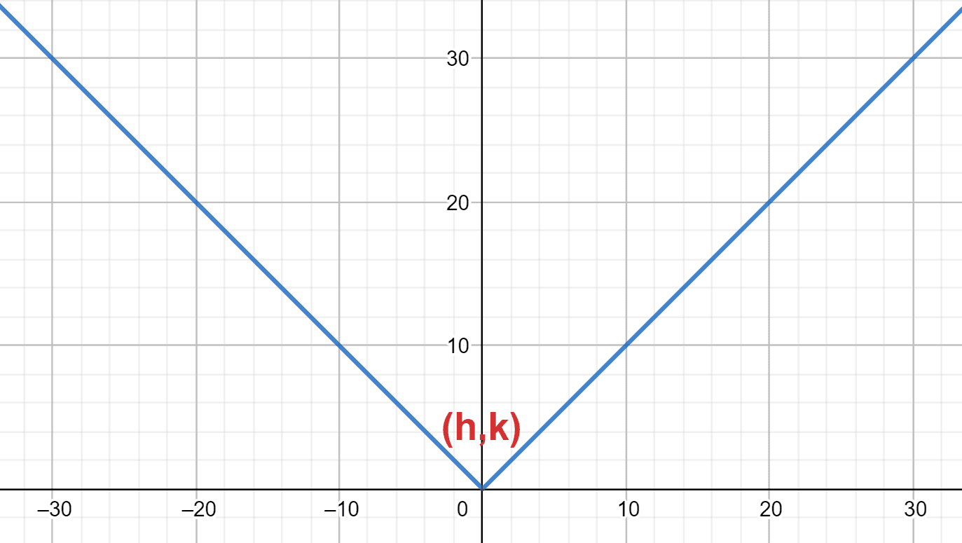
Identifying Key Components: With my function in hand, I identify critical points (points where the function’s graph has a peak or trough), asymptotes (lines that the graph approaches but never touches), and the y-intercept, where the graph crosses the y-axis.
Creating a Table of Values: Next, I often find it helpful to make a table of selected x-values and their corresponding y-values from the function. These are my ordered pairs in the format $(x, y)$.
| x | f(x) |
|---|---|
| -2 | |
| -1 | |
| 0 | |
| 1 | |
| 2 |
Plotting Points: Once I’ve calculated the y-values, I fill them in the table and then plot these points on my coordinate plane. Each point on the function’s graph represents an x-value from the domain with its corresponding y-value as the output.
Drawing the Graph: After plotting enough points, I connect them with a smooth line or curve. It’s important to consider the shape of the graph indicated by the function type, like linear, quadratic, or exponential.
If my function describes a linear relation, I’ll only need two points to draw a straight line. However, with non-linear functions, the more points I plot, the more accurate my graph will be.
By carefully following these steps, I can accurately sketch any function and gain a visual understanding of its behavior.
Using Technology to Graph Functions
When I graph functions, I find that utilizing technology streamlines the process. A variety of tools, including apps and web-based platforms, are available for this purpose. I’ll focus on how you can use these technologies effectively to graph mathematical functions.
Web-Based Graphing Calculators:
I often use online graphing calculators for their convenience. Platforms like Desmos are accessible directly from a web browser, which means there’s no need to download software. These tools are usually free and offer a wide range of functions, from plotting trigonometric functions to exploring more complex algebraic equations.
Features to Look For:
- Graphing Capabilities: The ability to plot multiple functions simultaneously.
- Sliders: Integrate dynamic variables into your graphs.
- Animation: Visualize how graphs change over time or with different parameters.
Downloading vs. Online Access:
Some graphing software requires a download, but I prefer online tools because they often have fewer loading times and don’t consume local storage. The web-based tools are also regularly updated with new features and improvements.
Importing External Resources:
The ability to load external data is an added benefit. For intricate datasets, this feature can be a huge time-saver.
Using Apps:
If I need to graph functions on the go, I use apps available for tablets and smartphones. They work similarly to web-based tools but are optimized for touch interfaces.
Considerations When Using Technology:
| Feature | Importance |
|---|---|
| User Interface | Must be clear and simple |
| Accessibility | Should be web-based |
| Cost | Preferably free |
| Learning Resources | Helpful for beginners |
Remember that when using online tools, ensure your internet connection is stable, and be aware that some platforms might be restricted depending on your web filter settings. A free trial is often offered, which allows you to test full features before committing, especially for premium tools.
Analyzing Graphs for Function Properties
When I graph a function, my goal is to interpret and identify its key properties, which reveal the behavior of the function. Let me walk you through the steps I follow to analyze these graphs:
Critical Points:
I look for points where the function’s derivative is zero or undefined, as these are potential maxima, minima, or points of inflection.
Y-Intercept:
I find the y-intercept by setting (x = 0) and evaluating the function, (f(0)), which tells me where the function crosses the y-axis.
Asymptotes:
I determine asymptotes to understand the function’s behavior at extreme values. If the function grows without bound near a certain value of (x), or if it approaches a certain value of (y) as (x) goes to infinity, these are likely asymptotes.
Curve Behavior:
I study the intervals where the function increases or decreases and the concavity of the curve. This helps me see the overall shape and direction of the graph.
| Property | What to Look For |
|---|---|
| Critical Points | Where (f'(x) = 0) or is undefined |
| Y-Intercept | The point where (x = 0) |
| Asymptotes | Values that (f(x)) approaches as (x) or (y) goes to infinity |
| Curve | Increasing/Decreasing intervals and concavity |
By analyzing these properties thoroughly, I can sketch a representative graph that captures the essence of the function’s behavior. Remember, always cross-reference your findings with the actual function to ensure the graph is accurate.
Examples and Engineering Applications
When I approach the task of graphing a function, I consider it in two phases: example-setting and real-world application. For illustration, let’s consider a basic linear function, where I want to determine its graph.
The general form of such a function is ( y = mx + b ), where ( m ) represents the slope and ( b ) represents the y-intercept. When I plot this function, I start by marking the y-intercept on the graph, and from there, I use the slope to determine the next points.
In engineering, graphing functions become a powerful tool to model and analyze physical systems.
For instance, Hooke’s Law in mechanical engineering is defined by ( F = kx ), which I can represent on a graph with force (F) on the y-axis and displacement (x) on the x-axis. This visual representation helps me understand how the spring will react under various forces.
Electrical engineering provides another example where function graphs are indispensable. Ohm’s Law, ( V = IR ), which defines the relationship between voltage (V), current (I), and resistance (R), can also be plotted. I can swiftly determine how changing one variable affects the others just by looking at the graph.
The domains of these functions are critical because they inform me of the input values that the function can accept. For practical engineering functions, the domain is often determined by physical constraints, and I ensure the functions are unblocked and accessible across all relevant values.
A quick reference I’ve created:
| Function Type | Domain Example |
|---|---|
| Hooke’s Law | ( $x \geq 0$ ) |
| Ohm’s Law | ( $I \geq 0 $) |
Websites like TeachEngineering and Khan Academy offer extensive resources where I can reinforce my understanding and practice graphing techniques. Using these online platforms, I can ensure my skills stay sharp for both theoretical and practical applications.
Conclusion
I’ve walked you through the essential steps to graph a function, from identifying critical points to plotting and drawing the curve.
Remember that practice is key in mastering this skill—so grab some graph paper and try graphing various functions to get comfortable with the process. Whether you’re dealing with a linear function, where your graph is a straight line given by ( y = mx + b ), or a more complex polynomial, the fundamentals remain the same.
Always start by finding critical points, such as intercepts and peaks. Highlight these on your graph first, as they provide a roadmap for the shape of your function.
Next, consider the behavior of the function as it moves towards infinity or negative infinity, and indicate if there are any asymptotes to be aware of. Then, smoothly connect your points with a curve that reflects the function’s rate of change.
For iterative learning, check your work with a graphing calculator or software to see if your hand-drawn graph aligns with the computed one. This comparison can be a great learning tool and confidence booster.