JUMP TO TOPIC

We examine the integral of a constant, which is a fundamental tool that plays a pivotal role in the grand scheme of mathematical concepts. It allows us to tackle problems involving areas, volumes, central points, and many other situations where adding infinitely many infinitesimal quantities is required.
One of the simplest cases of integration, yet extremely important, is the integral of a constant. This article will explore this concept’s significance, interpretation, and application in various fields.
Defining the Integral of a Constant
A constant is a number whose value is fixed. In calculus, the integral of a constant, denoted as ∫k dx where k is a constant, is straightforward to calculate: it is simply kx + C, where x is the variable of integration, and C is the constant of integration. This represents an indefinite integral, or antiderivative, meaning the family of functions that differentiate to give the original constant function.
Why does this make sense? Let’s break it down. The fundamental concept behind integration is finding the area under a curve. The graph is a horizontal line when the curve is defined by y = k, a constant function.
The area under this line between any two points, from 0 to x, is a rectangle with width x and height k. Therefore, the area is k*x, aligning perfectly with the formula for the integral of a constant.
The constant of integration, C, appears because the differentiation process removes constants, meaning that the original function could have added any constant without changing the derivative. Therefore, when we find an antiderivative, we account for this possible constant by including ‘+ C’ in the integral.
Graphical Representation
The integral of a constant function can be understood graphically as the area under the curve of the constant function over an interval.
A constant function is a horizontal line on the xy-plane at y = c, where c is a constant. Let’s say we’re interested in the definite integral of a constant c over an interval [a, b].
Constant Function
Draw the line y = c. A horizontal line will pass through the y-axis at the point (0, c). Below is the graphical representation of a generic constant function.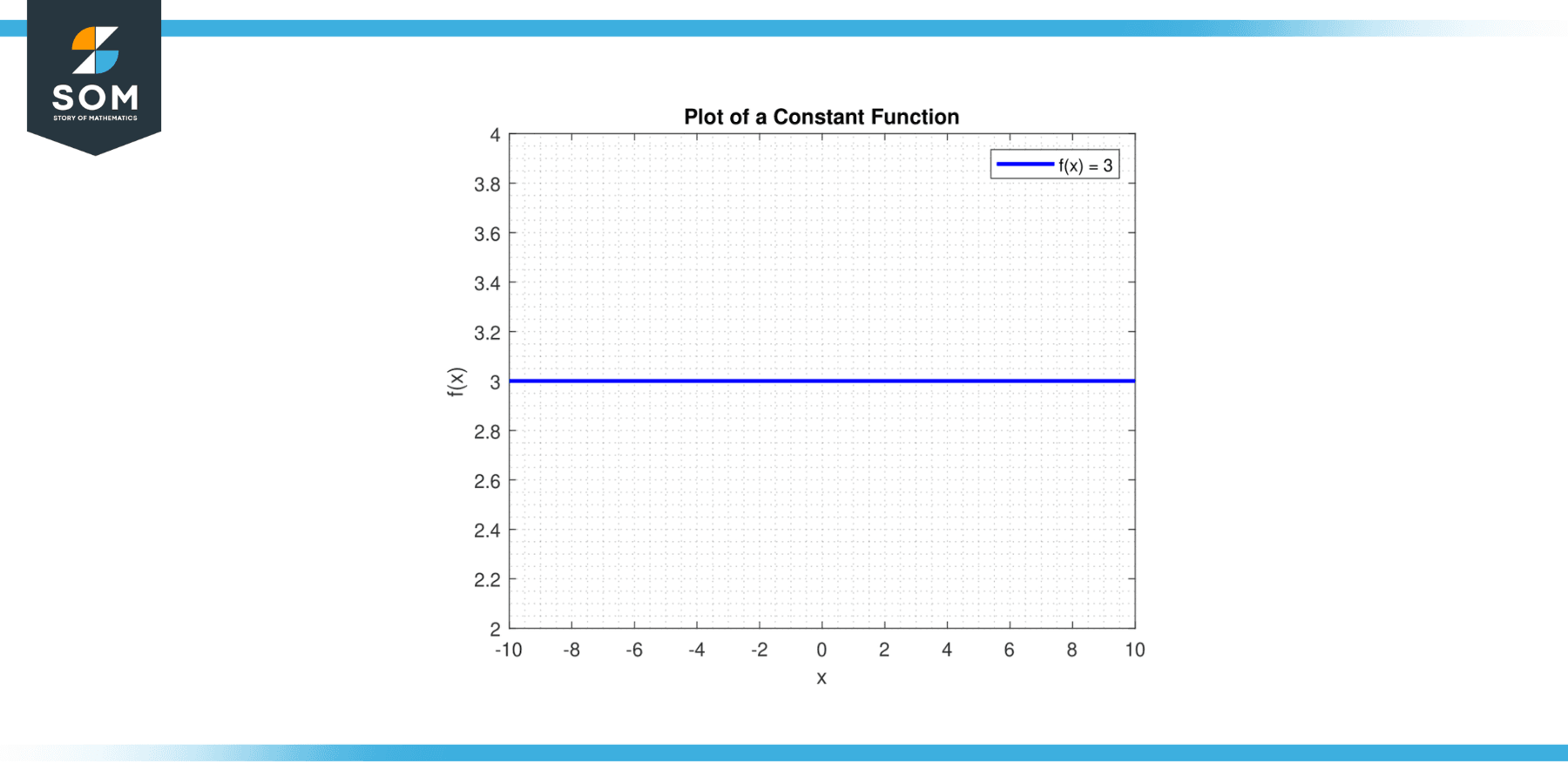
Figure-1.
Interval
On the x-axis, mark the points corresponding to a and b.
Area
The definite integral ∫c dx from a to b corresponds to the rectangle area formed by the horizontal line y = c, the x-axis (y = 0), and the vertical lines x = a and x = b. This rectangle has a width (b – a) and height of c, so its area is c * (b – a), which matches the formula for the integral of a constant.
In the case of the indefinite integral, or antiderivative, of a constant, the graph is a bit different: Below is the graphical representation of the shaded area for a generic constant function.
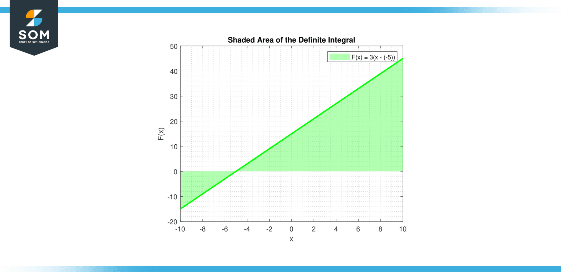
Figure-2.
Indefinite Integral
The indefinite integral of a constant c is given by ∫c dx = cx + C, which is the equation of a line. The line has slope c, and y-intercept C. Below is the graphical representation of the definite integral for a generic constant function.
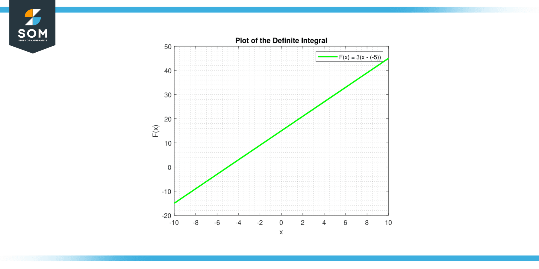
Figure-3.
Line Graph
Draw the line corresponding to y = cx + C. For different values of C, you get a family of parallel lines. These lines are solutions to the differential equation dy/dx = c.
In both cases, the graphical representation provides a visual interpretation of the integral of a constant, whether as the area under a curve (definite integral) or as a family of functions (indefinite integral). Below is the graphical representation of a generic line graph for the integration of a constant function.
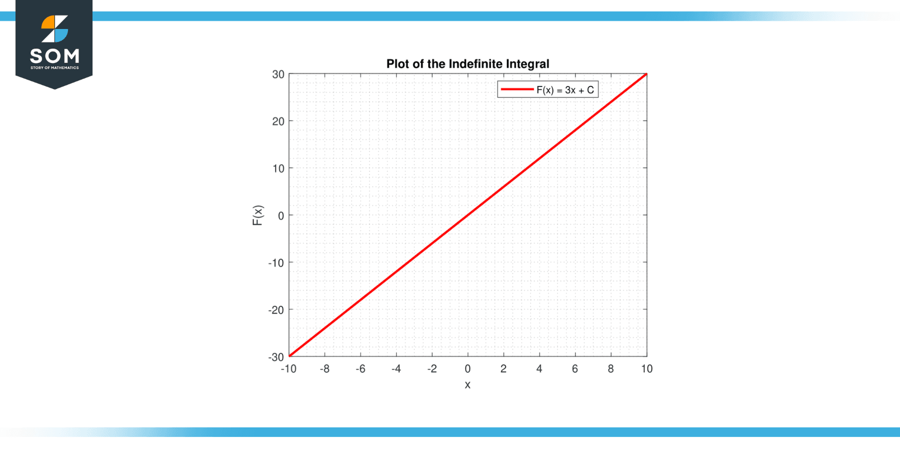
Figure-4.
Properties of Integral of a Constant
The integral of a constant, while being a straightforward concept, indeed possesses some fundamental properties. Let’s explore these properties in detail:
Linearity
The integral of a sum or difference of constants is equal to the sum or difference of their integrals. Mathematically, this is expressed as ∫(a ± b) dx = ∫a dx ± ∫b dx, where a and b are constants.
Scalability
The integral of constant times a function equals the constant times the integral of the function. For example, if we consider ∫cf(x) dx (where c is a constant and f(x) is a function of x), it can be simplified to c∫f(x) dx. This property is particularly useful when dealing with integrals involving constants.
Definite Integral and Area
If you compute the definite integral of a constant k over an interval [a, b], the result is k(b – a). This is equivalent to the area of a rectangle with base (b – a) and height k. This geometric interpretation of the integral of a constant as an area is quite useful.
The integral of Zero
The integral of zero is a constant, often represented by C. This makes sense as the antiderivative of a zero function (a horizontal line at y = 0) would be a constant function.
Indefinite Integral or Antiderivative
The indefinite integral of a constant k, denoted as ∫k dx, equals kx + C, where x is the variable of integration, and C is the constant of integration or the arbitrary constant. This is essentially saying that a constant function has a linear antiderivative.
Application to Differential Equations
When dealing with differential equations, the integral of a constant often appears when a derivative is equal to a constant, leading to a solution that is a linear function.
These properties are intrinsic to the nature of the integral of a constant and shape our understanding of many problems in calculus. Recognizing these properties can help tackle complex problems in mathematics and its applications.
Applications
While seemingly a simple concept, the integral of a constant has a broad range of applications across various fields. Let’s explore how it applies in different disciplines:
Physics
In physics, the integral of a constant often arises in scenarios where some quantity changes at a constant rate. For instance, if an object is moving at a constant velocity, the displacement (distance traveled) is the integral of the velocity, which is a constant. Similarly, if a force applied on an object is constant, the change in momentum (impulse) is the integral of the force.
Economics and Business
In economics, the integral of a constant can be used to model scenarios where a rate is constant over time. For example, if a company sells a product at a constant rate, the total revenue over a given period is the integral of the sales rate. Similarly, if a business has a constant rate of expenditure, the total cost over a period is the integral of the expenditure rate.
Environmental Science
In environmental science, the integral of a constant can be used to calculate total quantities from constant rates. For example, if a pollutant is being constantly released into an ecosystem, the total amount added over a period is integral to the emission rate.
Engineering
In engineering, the integral of a constant finds applications in systems where a constant input leads to a linearly changing output. For example, in control systems or signal processing, a system’s response to a constant input can often be determined using the concept of the integral of a constant.
Mathematics
In mathematics, the integral of a constant is a fundamental concept in calculus and is often used in solving differential equations where the derivative is a constant. This concept is also central to the Fundamental Theorem of Calculus, which connects differentiation and integration.
The integral of a constant is a foundational concept with diverse applications. In all these contexts, the underlying idea is the same: integrating a constant over an interval gives the total quantity that accumulates when something changes at a constant rate.
Exercise
Example 1
Evaluate the integral ∫5 dx.
Solution
By definition, the integral of a constant k with respect to x is
kx + C
Therefore, ∫5 dx = 5x + C.
Example 2
Evaluate the integral ∫3 dx from 0 to 4.
Solution
This is a definite integral of the constant 3 from 0 to 4. By the properties of the integral of a constant, this is
3(4-0) = 12
Example 3
Evaluate the integral ∫0 dx.
Solution
The integral of zero is a constant, so
∫0 dx = C
Example 4
If ∫k dx = 2x + 3 for all x, what is the value of k?
Solution
The integral of a constant k is kx + C. Comparing this with 2x + 3, and we see that k = 2.
Example 5
Find the area under the graph of y = 7 from x = 1 to x = 5.
Solution
The area under a constant function y = k from x = a to x = b is the integral of the constant from a to b, so the area is
A = $\int_{1}^{5}$ 7 dx
A = 7 * (5-1)
A = 28 square units
Example 6
Evaluate the integral ∫(-6) dx from -2 to 3.
Solution
This is the integral of the constant -6 from -2 to 3, which is
$\int_{-2}^{3}$ 6 dx = -6(3 – (-2))
$\int_{-2}^{3}$ 6 dx = -6 * 5
$\int_{-2}^{3}$ 6 dx = -30
Example 7
If a car moves at a constant speed of 60 km/h, how far does it travel in 2 hours?
Solution
Distance is the integral of speed over time. Therefore, the distance traveled is ∫60 dt from 0 to 2
$\int_{0}^{2}$ 60 dx = 60(2-0)
$\int_{0}^{2}$ 60 dx = 120 km
Example 8
Given that the function F(x) is an antiderivative of 4 and F(1) = 7, find F(x).
Solution
An antiderivative of a constant k is kx + C. So F(x) = 4x + C. To find C, we use the condition
F(1) = 7
Substituting these values gives us
7 = 4 * 1 + C
So C = 3. Therefore, F(x) = 4x + 3.
All images were created with MATLAB.