Welcome to an illuminating exploration of the integration of csc(x)! In the realm of calculus, the integral of the cosecant function holds intriguing properties and applications. This article delves into the world of csc(x) integration, where we will unlock its secrets and reveal the techniques required to tackle its challenges.

From the fundamental concepts of trigonometry to advanced calculus, we will traverse the intricacies of finding the antiderivative of csc(x). Prepare to unravel the mysteries and gain a deeper understanding of this fascinating topic as we embark on a journey through the integral of csc(x).

Interpreting the csc Function

The csc function, also known as the cosecant function, is a trigonometric function that relates to the properties of a right triangle. It is the reciprocal of the sine function and is defined as the ratio of the hypotenuse to the length of the side opposite a given angle in a right triangle.

In more formal mathematical terms, the csc function is defined as follows:

csc(θ) = 1 / sin(θ)

Here, θ represents the angle in radians or degrees for which you want to evaluate the cosecant function.

The csc function can be thought of as the ratio of the length of the hypotenuse to the length of the side opposite the given angle. In a right triangle, the hypotenuse is the side opposite the right angle, while the side opposite the given angle is the side that is not the hypotenuse.

The csc function is periodic, meaning it repeats its values in a regular pattern as the angle increases or decreases. The function has vertical asymptotes at multiples of π (or 180 degrees), where the value of the function approaches positive or negative infinity, depending on the quadrant.

The range of the csc function is all real numbers except for values between -1 and 1, inclusive. The graph of the csc function resembles a series of curves that approach the vertical asymptotes as the angle approaches the values of the asymptotes.

The csc function is commonly used in various branches of mathematics and engineering, especially in trigonometry, calculus, and physics. It helps in solving problems involving angles, triangles, and periodic phenomena.

It’s worth noting that the csc function can also be expressed in terms of the unit circle, complex numbers, and exponential functions, providing alternative representations and ways of calculating its values.

Graphical Representation

The graphical representation of the cosecant function, csc(x), provides insights into its behavior, periodicity, and asymptotic properties. Here’s a discussion of the key features and characteristics of the graph:

Periodicity

The cosecant function is periodic, meaning it repeats its values in a regular pattern as the angle increases or decreases. The period of csc(x) is 2π (or 360 degrees). This means that the function has the same value at x and x + 2π, for any real value of x.

Vertical Asymptotes

The graph of csc(x) has vertical asymptotes where the function is undefined. These occur when sin(x) equals zero, which happens at x = nπ, where n is an integer. At these points, the value of csc(x) approaches positive or negative infinity, depending on the quadrant.

Range

The range of the cosecant function is all real numbers except for values between -1 and 1, inclusive. This is because the reciprocal of a number between -1 and 1, when multiplied by a positive value, becomes greater than 1, and when multiplied by a negative value, becomes less than -1.

Shape and Symmetry

The graph of csc(x) consists of a series of curves that approach the vertical asymptotes as the angle approaches the values of the asymptotes. These curves repeat symmetrically on either side of the asymptotes. The graph is symmetric about the vertical lines x = (2n + 1)π/2, where n is an integer.

Behavior at the Vertical Asymptotes

As x approaches the vertical asymptotes (x = nπ), the graph of csc(x) approaches positive or negative infinity. The function has vertical tangent lines at these points, representing an abrupt change in the slope of the graph.

Points of Interest

Some notable points on the graph include the maximum and minimum points. The maximum points occur when the sine function reaches its maximum value of 1, and the minimum points occur when the sine function reaches its minimum value of -1. These extrema are located between the vertical asymptotes.

Graph Transformations

The graph of csc(x) can be transformed using standard transformations such as translations, dilations, and reflections. These transformations can shift the position of the graph horizontally or vertically, stretch or compress it, or reflect it across the x-axis.

It’s important to note that the scale and specific characteristics of the graph can vary depending on the chosen interval or viewing window. However, the overall shape, periodicity, vertical asymptotes, and behavior of csc(x) remain consistent across different representations.

To get a better visual understanding of the cosecant function, below we present the graphical representation of csc function in Figure-1.

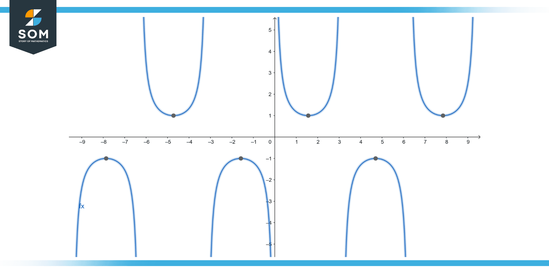
Figure-1. Generic csc function.

Integration of the csc Function

The integration of csc(x), also known as the antiderivative or integral of the cosecant function, involves finding a function whose derivative yields csc(x). Mathematically, the integral of csc(x) can be represented as ∫csc(x) dx, where the integral symbol (∫) signifies the integration process, csc(x) represents the cosecant function, and dx denotes the differential variable concerning which integration is performed.

Solving this integral requires employing various integration techniques such as substitution, trigonometric identities, or integration by parts. By determining the antiderivative of csc(x), we can ascertain the original function that, when differentiated, results in csc(x). Understanding the integration of csc(x) is crucial in diverse mathematical applications and problem-solving scenarios.

To get a better visual understanding of the integration of the cosecant function, below we present the graphical representation of the integration of csc function in Figure-2.

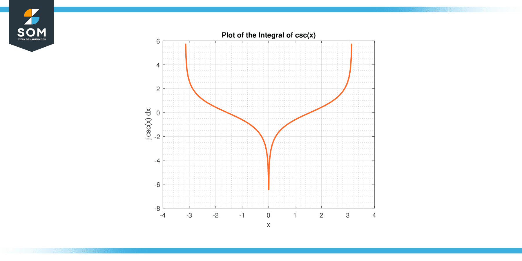
Figure-2. Integration of csc function.

Properties

The integral of the cosecant function, ∫csc(x) dx, has several properties and can be expressed in different forms depending on the context and the techniques used for integration. Here are the main properties and forms associated with the integration of csc(x):

Basic Integral

The most common form of the integral of csc(x) is given by: ∫csc(x) dx = -ln|csc(x) + cot(x)| + C Here, C represents the constant of integration, and ln denotes the natural logarithm. This form is derived by rewriting csc(x) in terms of sine and cosine and using integration techniques such as substitution or integration by parts.

Integration Bounds

When evaluating the integral of csc(x) over a specific interval [a, b], it’s important to consider the behavior of the function within that interval. The cosecant function is undefined when sin(x) equals zero, which occurs at x = nπ, where n is an integer. If any of the integration bounds lie at these points, the integral is not defined.

Improper Integrals

If the integration bounds extend to the points where the cosecant function is undefined (x = nπ), the integral is considered improper. In such cases, special techniques like Cauchy principal value or limit evaluation may be used to compute the integral.

Symmetry

The cosecant function is an odd function, meaning it exhibits symmetry about the origin (x = 0). Consequently, the integral of csc(x) over a symmetric interval centered at the origin is zero: ∫[-a, a] csc(x) dx = 0

Trigonometric Identities: Trigonometric identities can be employed to simplify or transform the integral of csc(x). Some commonly used identities include:

csc(x) = 1/sin(x) csc(x) = cos(x)/sin(x) csc(x) = sec(x)cot(x) By applying these identities and other trigonometric relationships, the integral can sometimes be rewritten in a more manageable form.

Integration Techniques

Due to the complexity of the integral of csc(x), various integration techniques may be employed, such as: Substitution: Substituting a new variable to simplify the integral. Integration by Parts: Applying integration by parts to split the integral into product terms. Residue Theorem: Complex analysis techniques can be utilized to evaluate the integral in the complex plane. These techniques may be combined or used iteratively depending on the complexity of the integral.

Trigonometric Substitution

In certain cases, it may be beneficial to use trigonometric substitutions to simplify the integral of csc(x). For example, substituting x = tan(θ/2) can help convert the integral into a form that can be evaluated more easily.

It’s important to note that the integral of csc(x) can be challenging to compute in some cases, and closed-form solutions may not always be possible. In such situations, numerical methods or specialized software can be employed to approximate the integral.

Ralevent Formulas 

The integration of the cosecant function, ∫csc(x) dx, involves several related formulas that are derived using various integration techniques. Here are the main formulas associated with the integration of csc(x):

Basic Integral

The most common form of the integral of csc(x) is given by: ∫csc(x) dx = -ln|csc(x) + cot(x)| + C

This formula represents the indefinite integral of the cosecant function, where C is the constant of integration. It is obtained by rewriting csc(x) in terms of sine and cosine and using integration techniques such as substitution or integration by parts.

Integral with Absolute Values

Since the cosecant function is not defined at points where sin(x) = 0, the absolute value is often included in the integral to account for the change in sign when crossing those points. The integral can be expressed as: ∫csc(x) dx = -ln|csc(x) + cot(x)| + C, where x ≠ nπ, n ∈ Z.

This formula ensures that the integral is well-defined and handles the singularity of the cosecant function.

Integral using Logarithmic Identities

By employing logarithmic identities, the integral of csc(x) can be written in alternative forms. One such form is: ∫csc(x) dx = -ln|csc(x) + cot(x)| + ln|tan(x/2)| + C.

This formula uses the identity ln|tan(x/2)| = -ln|cos(x)|, which simplifies the expression and provides an alternative representation of the integral.

Integral with Hyperbolic Functions

The integral of csc(x) can also be expressed using hyperbolic functions. By substituting x = -i ln(tan(θ/2)), the integral can be written as: ∫csc(x) dx = -ln|cosec(x) + cot(x)| + i tanh⁻¹(cot(x)) + C.

Here, tanh⁻¹ represents the inverse hyperbolic tangent function. This formula provides a different perspective on the integration of the cosecant function using hyperbolic trigonometric functions.

Integral with Complex Analysis

Complex analysis techniques can be employed to evaluate the integral of csc(x) using the residue theorem. By considering the contour integral around a semicircular path in the complex plane, the integral can be expressed as a sum of residues at singularities. This approach involves integrating along the branch cut of the logarithm and utilizing complex logarithmic identities.

It’s worth noting that the integral of csc(x) can be challenging to compute in some cases, and closed-form solutions may not always be possible. In such situations, numerical methods or specialized software can be employed to approximate the integral.

Applications and Significance

The integration of the cosecant function, ∫csc(x) dx, has various applications in different fields, including mathematics, physics, engineering, and signal processing. Here are some notable applications:

Calculus and Trigonometry

In mathematics, the integration of csc(x) is an important topic in calculus and trigonometry. It helps in solving problems related to evaluating definite integrals involving trigonometric functions and in finding antiderivatives of functions containing the cosecant function.

Physics

The integration of csc(x) finds applications in various areas of physics, particularly in wave phenomena and oscillations. For example, in the study of periodic motion and vibrations, the integral of csc(x) can be used to calculate the period, frequency, amplitude, or phase of a wave.

Harmonic Analysis

In the field of harmonic analysis, the integration of csc(x) is utilized to analyze and synthesize complex periodic signals. By understanding the properties of the integral of csc(x), researchers can study the spectral characteristics, frequency components, and phase relationships of signals in fields like audio processing, music theory, and signal modulation.

Electromagnetism

The integral of csc(x) has applications in electromagnetic theory, specifically when dealing with problems involving diffraction, interference, and propagation of waves. These concepts are crucial in the study of optics, antenna design, electromagnetic waveguides, and other areas related to the behavior of electromagnetic waves.

Control Systems Engineering

In control systems engineering, the integration of csc(x) is used to analyze and design systems with periodic or oscillatory behavior. Understanding the integral of csc(x) allows engineers to model and control systems that exhibit cyclic patterns, such as electrical circuits, mechanical systems, and feedback control systems.

Applied Mathematics

In various branches of applied mathematics, the integration of csc(x) plays a role in solving differential equations, integral transforms, and boundary value problems. It contributes to finding solutions for mathematical models involving trigonometric phenomena, such as heat conduction, fluid dynamics, and quantum mechanics.

Analytical Chemistry

The integration of csc(x) is also relevant in analytical chemistry, particularly when determining concentrations and reaction rates. By applying techniques that involve the integration of csc(x), chemists can analyze and quantify the behavior of reactants and products in chemical reactions, as well as calculate reaction kinetics and equilibrium constants.

These are just a few examples of the diverse applications of the integration of csc(x) across various fields. The cosecant function and its integral have a wide range of practical uses, contributing to the understanding and analysis of phenomena involving periodic behavior, waves, and oscillations.

Exercise 

Example 1

f(x) = ∫csc(x) dx

Solution

We can start by using the identity csc(x) = 1/sin(x) to rewrite the integral:

∫csc(x) dx = ∫(1/sin(x)) dx

Next, we can use substitution to simplify the integral. Let u = sin(x), then du = cos(x) dx. Rearranging, we have:

dx = du/cos(x)

Substituting these values, the integral becomes:

∫(1/sin(x)) dx = ∫(1/u)(du/cos(x)) = ∫(du/u) = ln|u| + C = ln|sin(x)| + C

Therefore, the solution to ∫csc(x) dx is ln|sin(x)| + C, where C is the constant of integration.

Example 2

f(x) = ∫csc²(x) dx.

Solution

To solve this integral, we can use a trigonometric identity: csc²(x) = 1 + cot²(x)

The integral can be rewritten as:

∫csc²(x) dx = ∫(1 + cot²(x)) dx

The first term, ∫1 dx, integrates to x. For the second term, we use the identity cot²(x) = csc²(x) – 1. Substituting, we have:

∫cot²(x) dx = ∫(csc²(x) – 1) dx = ∫csc²(x) dx – ∫dx

Combining the results, we get:

∫csc²(x) dx – ∫csc²(x)dx = x – x + C = C

Therefore, the solution to ∫csc²(x) dx is simply the constant C.

Example 3

f(x) = ∫csc²(x) cot(x) dx.

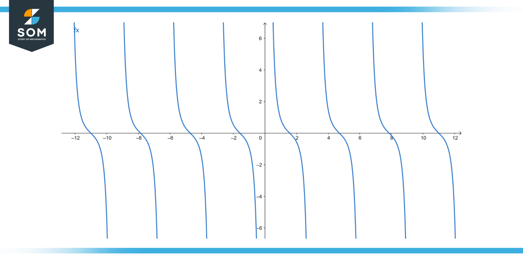
Figure-4.

Solution

We can rewrite the integral using the identity csc²(x) cot(x) = (1 + cot²(x)) * (csc²(x)/ sin(x)):

∫csc²(x) cot(x) dx = ∫(1 + cot²(x)) * (csc^2(x) / sin(x)) dx

Next, we can use substitution, letting u = csc(x), which gives du = -csc(x) cot(x) dx. Rearranging, we have:

-du = csc(x) cot(x) dx

Substituting these values, the integral becomes:

∫(1 + cot²(x)) * (csc²(x) / sin(x)) dx = -∫(1 + u²) du = -∫du – ∫u² du = -u – (u³/3) + C = -csc(x) – (csc³(x)/3) + C

Therefore, the solution to ∫csc²(x) cot(x) dx is -csc(x) – (csc³(x)/3) + C, where C is the constant of integration.

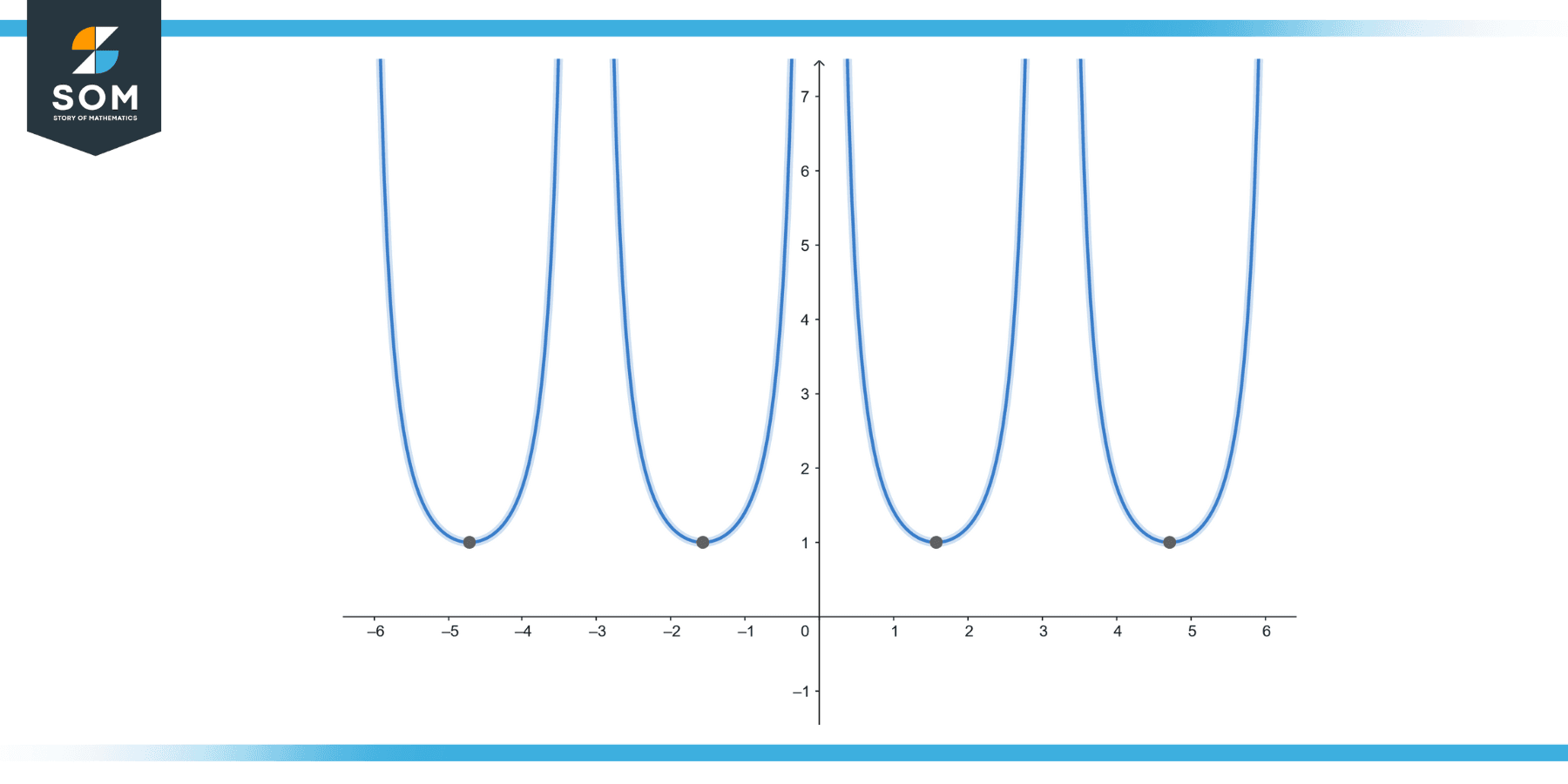
Example 4

f(x) = ∫csc³(x) dx.

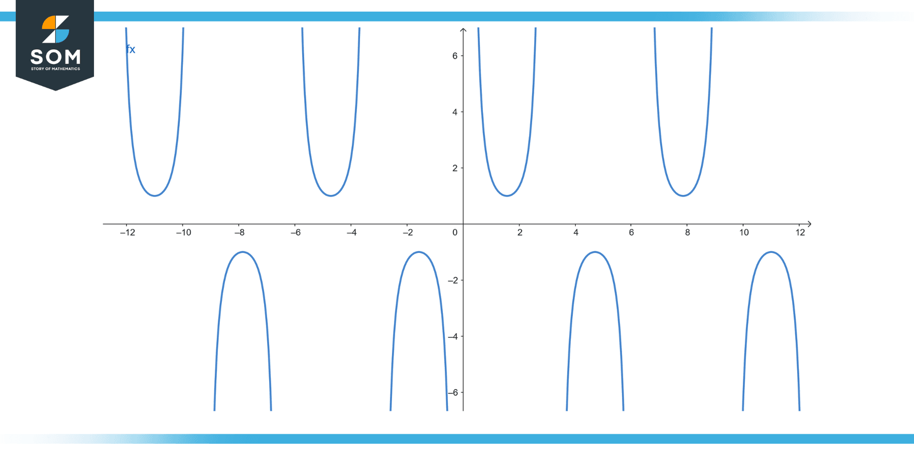
Figure-5.

Solution

We can rewrite the integral using the identity csc³(x) = csc(x) * (csc²(x)) = csc(x) * (1 + cot²(x)):

∫csc³(x) dx = ∫csc(x) * (1 + cot²(x)) dx

Using substitution, let u = csc(x), which gives du = -csc(x) cot(x) dx. Rearranging, we have:

-du = csc(x) cot(x) dx

Substituting these values, the integral becomes:

∫csc(x) * (1 + cot²(x)) dx = -∫(1 + u²) du = -∫du – ∫u² du = -u – (u³/3) + C = -csc(x) – (csc³(x)/3) + C

Therefore, the solution to ∫csc³(x)dx is -csc(x) – (csc³(x)/3) + C, where C is the constant of integration.

All images were created with GeoGebra and MATLAB.