JUMP TO TOPIC
Inverse variation equations represent a captivating class of mathematical relationships that embody a distinct form of interdependence. When an inverse variation equation links two variables, an increase in one leads to a corresponding decrease in the other, and vice versa.
This article will explore the mathematical elegance and practical importance inherent to inverse variation equations.
Defining Inverse Variation Equation
An inverse variation equation is a relationship between two variables such that their product is a constant. It is also known as inverse proportionality or inverse variation. In mathematical terms, if two variables x and y are inversely proportional, it can be written as:
xy = k
where:
- x and y are the variables,
- k is a non-zero constant.
This equation expresses that when x increases, y decreases so that their product remains the same, and vice versa. For instance, if you were to double x, you would need to halve y to maintain the same product k.
The equation can be rearranged to make y the subject:
y = k / x
This shows that y equals a constant divided by x, which underlines the idea of inverse variation: y decreases as x increases, and vice versa.
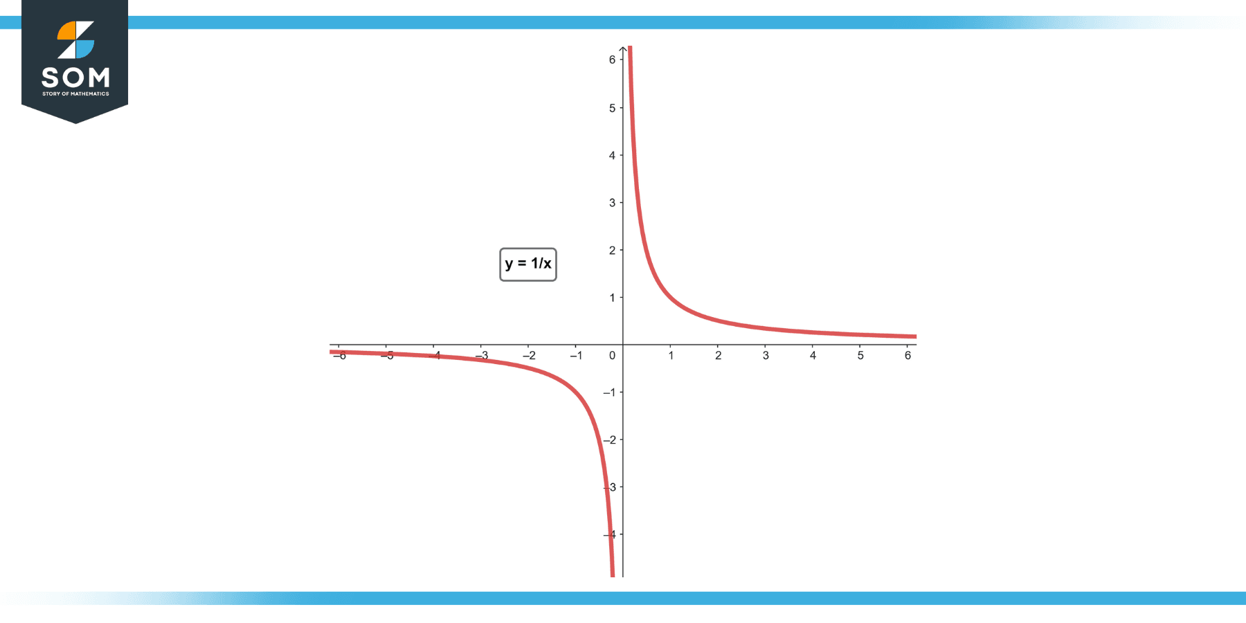
Figure-1.
Inverse variation equations describe many real-world phenomena where one quantity decreases when another increases, such as the speed required to travel a certain distance in a fixed amount of time or the light intensity as you move away from a source.
Properties of Inverse Variation Equation
An inverse variation equation, also known as an inverse proportionality equation, has several key properties. Understanding these characteristics can help you identify, work with, and apply inverse variation in various mathematical and real-world contexts.
Constant Product
The most fundamental property of inverse variation is that the product of the two variables is constant. If y varies inversely as x, then the product xy = k, where k is a non-zero constant. This means that as one variable increases, the other variable decreases so that its product remains constant.
Inverse Relationship
If y varies inversely as x, then as x increases, y decreases proportionally, and vice versa. This is where the term “inverse variation” comes from.
This relationship is represented by the equation y = k / x, where k is a non-zero constant. The equation signifies that as x increases, y decreases in a way that maintains the inverse variation relationship.
Non-linearity
Inverse variation is indeed a type of non-linear relationship between two variables. Unlike in a linear relationship, where the graph forms a straight line, the graph of an inverse variation equation forms a hyperbola.
A hyperbola is a curved shape consisting of two separate branches, a characteristic feature of inverse variation. The hyperbolic nature of the graph demonstrates the inverse relationship between the variables and highlights the non-linear behavior of the equation.
Asymptotic behavior
The graph of an inverse variation equation indeed has two asymptotes. The x-axis (where y = 0) and the y-axis (where x = 0) are asymptotes. This means that the graph approaches these axes but never crosses them.
As x or y approaches zero, the value of the other variable becomes extremely large, and the graph gets closer and closer to the respective axis. The presence of asymptotes adds to understanding the behavior and limits of the inverse variation relationship.
Quadrants
The inverse variation equation graph is located in the first and third quadrants when k is positive and in the second and fourth quadrants when k is negative. This is because the product of x and y is always positive in the first and third quadrants and negative in the second and fourth quadrants.
The sign of k determines the orientation of the graph and the regions where the inverse variation relationship holds. Understanding the quadrants where the graph lies provides insights into the nature and characteristics of the inverse variation equation.
Zeroes
An inverse variation equation has no zeroes, as no x or y values can make the equation equal to zero. That’s because the constant k in the equation xy = k is non-zero.
Sign of Variables
In an inverse variation, the sign of x and y will always be the same if k is positive and different if k is negative.
These properties of inverse variation equations apply not only to abstract mathematical problems but also to a wide range of real-world scenarios, from the physics of light and sound to various principles in engineering and economics.
Ralevent Formulas
In inverse variation relationships, there are a couple of key formulas that are generally used:
Inverse Variation Formula
The main formula that defines inverse variation between two variables, x, and y, is expressed as:
xy = k
Here, k is a non-zero constant.
Reformatted Inverse Variation Formula
You can also express the inverse variation formula by isolating one variable, typically written as:
y = k / x
Here, y varies inversely with x. When x increases, y decreases, and vice versa.
Solving for the Constant, k
In many problems, you’ll be given x and y and asked to find the constant of variation, k. You can solve for k by rearranging the formula:
k = xy
Once you’ve found k, you can use it to find y for any given x or x for any given y.
Solving for Unknown Variables
If you’re given k and either x or y, you can solve for the unknown variable by rearranging the formula:
If given k and y, solve for x:
x = k / y
If given k and x, solve for y:
y = k / x
Exercise
Example 1
If y varies inversely as x, and y = 2 when x = 3, find the constant of variation, k.
Solution
We can find k using the formula:
k = x * y
So:
k = 2 * 3
k = 6
Example 2
Given the inverse variation equation x * y = 4, find y when x = 2.
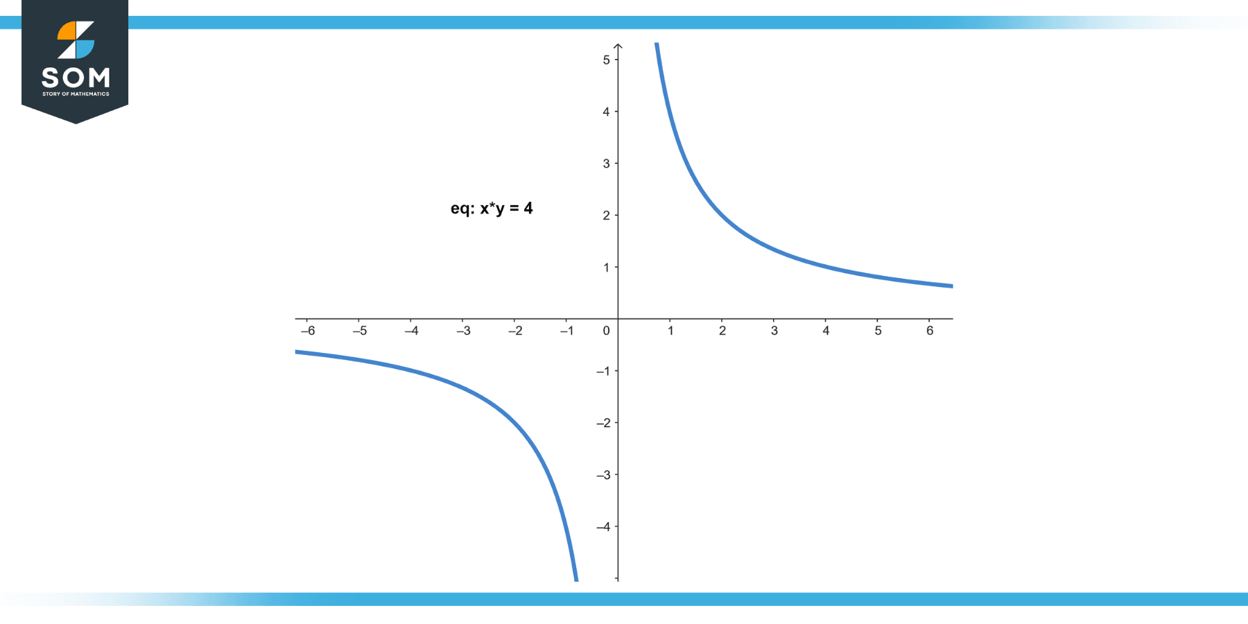
Figure-2.
Solution
Solve the equation for y by dividing both sides by x:
y = 4 / x
Substitute x = 2 we get:
y = 4 / 2
y = 2
Example 3
If y varies inversely as x, and y = 5 when x = 1, what is y when x = 10?
Solution
First, find the constant of variation:
k = xy
k = 5 * 1
k = 5
Then, using y = k / x, substitute k = 5 and x = 10, we get:
y = 5 / 10
y = 0.5
Example 4
If y varies inversely as x, and y = 3 when x = 4, find x when y = 1.
Solution
First, find the constant of variation:
k = xy
k = 3 * 4
k = 12
Then, using x = k / y, substitute k = 12 and y = 1, we get:
x = 12 / 1
x = 12
Example 5
If y varies inversely as x, and y = 2 when x = 5, find y when x = 15.
Solution
First, find the constant of variation:
k = xy
k = 2 * 5
k = 10
Then, using y = k / x, substitute k = 10 and x = 15, we get:
y = 10 / 15
y = 2/3
y ≈ 0.67
Example 6
Given the inverse variation equation x * y = 6, find x when y = 3.
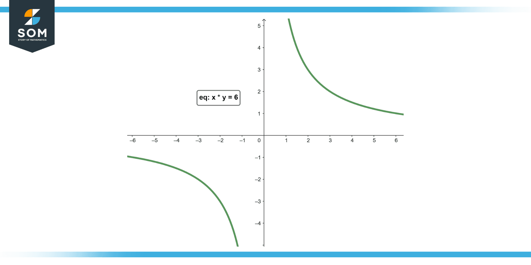
Figure-3.
Solution
Solve the equation for x by dividing both sides by y:
x = 6 / y
Substitute y = 3, we get:
x = 6 / 3
x = 2
Example 7
If y varies inversely as x, and y = 4 when x = 3, what is y when x = 9?
Solution
First, find the constant of variation:
k = xy
k = 4 * 3
k = 12
Then, using y = k / x, substitute k = 12 and x = 9, we get:
y = 12 / 9
y = 4/3
y ≈ 1.33
Example 8
If y varies inversely as x, and y = 6 when x = 2, find x when y = 3.
Solution
First, find the constant of variation:
k = xy
k = 6 * 2
k = 12
Then, using x = k / y, substitute k = 12 and y = 3, we get:
x = 12 / 3
x = 4
Applications
Physics – Gravitational and Electrostatic Forces
Both gravitational and electrostatic forces follow an inverse-square law, meaning the force decreases with the square of the distance. If you double the distance between two masses or charges, the gravitational or electrostatic force becomes a quarter of what it was.
The equations are:
F₉₉₍G₎ = G(m₁m₂)/r²
and
Fₑₗₑ = k(q₁q₂)/r²
where G and k are constants, m1, and m2 are the two masses, q1 and q2 are the two charges, and r is the distance between the masses or charges.
Chemistry – Ideal Gas Law
In the ideal gas law, the pressure P of a gas is inversely proportional to its volume V, assuming the temperature and amount of gas remain constant. This relationship is known as Boyle’s Law, and it is expressed as PV = k, where k is a constant.
According to Boyle’s Law, if a gas is compressed (decreasing volume), the pressure increases. Conversely, if a gas is allowed to expand (increasing volume), the pressure decreases.
Economics – Demand and Supply
The law of demand states that the price of a product is inversely proportional to the quantity demanded. In other words, as the price of a product increases, the demand decreases, and vice versa.
This law reflects the general consumer behavior where a higher price tends to discourage consumers from purchasing a larger quantity of the product, while a lower price stimulates demand.
Biology – Metabolic Rate
The relationship between an organism’s body size and metabolic rate often follows an inverse variation. For example, smaller animals tend to have higher metabolic rates than larger animals. Therefore, a mouse has a higher metabolic rate than an elephant.
Astronomy – Kepler’s Third Law
In astronomy, the square of the period of a planet’s orbit is inversely proportional to the cube of the semi-major axis of its orbit. This relationship is known as Kepler’s Third Law or the law of periods. It states that planets farther from the sun have longer orbital periods.
Engineering – Signal Processing
In signal processing, the frequency of a signal is inversely proportional to its period. If you increase the frequency of a signal, the period (or time taken for one complete cycle of the signal) decreases.
Ecology – Animal Population Dynamics
In ecology, the carrying capacity, representing the maximum population size an environment can sustain, often exhibits inverse variation with the per capita growth rate. This means that as an animal population approaches or exceeds the carrying capacity of its environment, the per capita growth rate decreases.
Computer Science – Parallel Processing
In parallel computing, the time taken to process a task can be inversely proportional to the number of processors, assuming perfectly parallelizable tasks. This relationship is based on the concept of parallel speedup. If you double the number of processors, the time taken to process the task has the potential to halve, thereby improving computational efficiency.
Historical Significance
Inverse variation, also known as inverse proportion or variation, has a rich historical background, much of which is intertwined with the development of mathematics and scientific thought over centuries.
Ancient Mathematics
The concept of inverse proportionality can be traced back to ancient mathematics. Ancient Greeks, including mathematicians like Euclid and Pythagoras, studied proportional relationships, though it’s unclear if they specifically dealt with inverse proportions.
Middle Ages and Renaissance
The principle of inverse variation gained explicit recognition during the Middle Ages and Renaissance periods. Scholars in the Middle East and Europe began developing the foundations of algebra, which led to a better understanding of proportional relationships, including inverse variation.
17th Century
The formulation of the inverse-square law in physics in the 17th century by Sir Isaac Newton was a crucial historical point for inverse variation. Newton’s Law of Universal Gravitation states that the force of gravity between two objects decreases with the square of the distance between them, a clear example of an inverse variation relationship.
18th Century
Swiss mathematician Leonhard Euler and others developed the formal mathematical notation and language we use today to describe inverse variation and many other mathematical relationships.
19th and 20th Centuries
In the 19th and 20th centuries, inverse variation became an important tool in numerous emerging scientific fields. For instance, it was used to describe phenomena such as electrical resistance in circuits, the behavior of gases in chemistry, and principles of economics like supply and demand.
In mathematics, inverse variation has emerged and evolved as part of the broader development of mathematical thought. From early explorations of proportion to the sophisticated mathematical languages of modern science, inverse variation has proven to be a vital tool in describing the world around us.
All images were created with GeoGebra.