JUMP TO TOPIC
In the intricate field of mathematics, few topics can be as fascinating, yet enigmatic, as orthogonal trajectories. Bridging the world of calculus, geometry, and differential equations, these intriguing curves serve as a testament to the harmonious symphony of mathematics.
This article endeavors to explore the concept of orthogonal trajectories, paths that intersect other curves at right angles, permeating diverse domains from physics to engineering. Here, we delve into their core principles, examine their real-world applications, and unravel the beauty they offer to mathematical understanding.
Whether you’re a budding mathematician, a seasoned scholar, or an inquisitive enthusiast, prepare for a journey into the captivating realm of orthogonal trajectories.
Definition of Orthogonal Trajectory
In the realm of mathematics, an orthogonal trajectory refers to a family of curves that intersect another family of curves at right angles (90 degrees), hence the term “orthogonal,” which is derived from the Greek words for “right” (ortho) and “angle” (gonia).
Each curve of one family intersects each curve of the other family at one point, and the angle of intersection is always 90 degrees. These trajectories are frequently applied in various scientific fields, including physics and engineering, where they often illustrate how different states or conditions evolve over time under the influence of a perpendicular or “orthogonal” force or function.
Below we present a generic representation of orthogonal trajectories in figure-1.
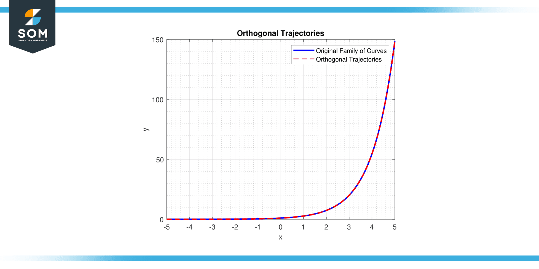
Figure-1.
Evaluating Orthogonal Trajectory
Evaluating or finding orthogonal trajectories involves solving a differential equation derived from the given family of curves. Here’s a step-by-step method to follow:
Step 1
Start with the equation of the given family of curves. This equation will typically involve a parameter (usually denoted by C or k) that differentiates one curve in the family from another.
Step 2
Differentiate the given equation with respect to x (or y, depending on the function) to find the slope of the curve, dy/dx. Remember to apply the chain rule, product rule, or quotient rule as needed.
Step 3
The orthogonal trajectories will intersect the original family of curves at a right angle, meaning the slope of the orthogonal trajectories will be the negative reciprocal of the original slope. So, take the negative reciprocal of the slope you calculated in step 2.
Step 4
This new slope will be a differential equation in terms of x and y. You now have to solve this differential equation. Depending on the complexity of the differential equation, you may be able to separate variables and integrate them, or you may need to use more advanced methods for solving differential equations.
Step 5
The solution to this differential equation will give you the family of orthogonal trajectories, typically involving a new integration constant.
Properties of Orthogonal Trajectory
Orthogonal trajectories have a number of distinct properties that arise due to their mathematical definition. These characteristics can have profound implications in both theoretical and applied contexts. Let’s delve into some of these properties:
Perpendicular Intersection
The principal and defining characteristic of orthogonal trajectories is that they intersect another family of curves at right angles, or 90 degrees. This is inherent in the word “orthogonal,” which originates from the Greek words ‘ortho,’ meaning right, and ‘gonia,’ meaning angle.
Uniform Intersection
Each curve in one family intersects each curve in the other at exactly one point, and this point is the same for all curves of a given family. This property can often simplify problems where it is necessary to understand the system’s behavior at these points of intersection.
Symmetry
Depending on the families of curves involved, orthogonal trajectories can often exhibit symmetry. This symmetry can be about an axis, a point, or another geometric entity. However, symmetry isn’t always a property of orthogonal trajectories – it depends on the specific families of curves in question.
Dynamic Behavior
In applied contexts such as physics and engineering, orthogonal trajectories can often describe the dynamic behavior of a system. They can represent the states or conditions evolving over time under the influence of a perpendicular or “orthogonal” force or function.
Solvability
Orthogonal trajectories can often be determined through the use of differential equations. If you know the equation of one family of curves, you can find the orthogonal trajectories by finding the solution to the differential equation that describes the orthogonal family. This typically involves taking the derivative of the given equation, negating it, and finding the reciprocal to determine the slope of the orthogonal trajectories.
Continuity
As long as the family of curves they are orthogonal to is continuous, orthogonal trajectories will also be continuous. They won’t suddenly break off or have gaps as they are mathematically tied to the other curves.
Diversity of Shapes
Orthogonal trajectories can take on a variety of forms and shapes depending on the original family of curves. They can be straight lines, curves, or even more complex figures. This is because the shape is dictated by the geometry and nature of the original family of curves and the restrictions of maintaining a right-angle intersection.
In essence, these properties give orthogonal trajectories a unique place within the mathematical landscape, offering insights into complex geometric relationships and the behavior of dynamic systems.
Applications
Orthogonal trajectories play a critical role in a variety of fields, from pure mathematics to applied physics and engineering, demonstrating the practical value of this mathematical concept. Let’s examine a few key applications across different domains:
Physics
In physics, orthogonal trajectories are often used in the study of electric and magnetic fields. The field lines in these fields can be viewed as a family of curves, and the equipotential lines (lines of equal potential) can be viewed as their orthogonal trajectories. The fact that these lines intersect at right angles can simplify calculations and improve understanding of the fields.
Engineering
Orthogonal trajectories find application in engineering fields such as control systems and signal processing. They can help in the analysis of systems where different parameters or states interact orthogonally, like in the design of orthogonal frequency-division multiplexing (OFDM) in telecommunications.
Fluid Dynamics
In fluid dynamics, the study of how fluids move, orthogonal trajectories can represent streamlined flow patterns. A streamline is a curve that is everywhere tangent to the velocity field of a fluid flow at a given instant. The pathlines (actual path traced by a given fluid particle) and streaklines (the locus of particles that were earlier present at a common point) can often be represented as orthogonal trajectories.
Computer Graphics
In computer graphics and image processing, orthogonal trajectories are used in the generation of orthogonal meshes, which are useful for texture mapping, 3D modeling, and solving partial differential equations numerically.
Biology
In biological contexts, orthogonal trajectories can be used to model various biological phenomena, such as the growth of biological tissues or the propagation of nerve impulses.
Chemistry
In chemistry, the concept of orthogonal trajectories can be used to represent phase-space trajectories in the study of dynamical systems, such as chemical reactions.
Mathematics
In mathematics itself, orthogonal trajectories are used in the study of differential equations, complex analysis, and other areas where families of curves are analyzed.
In summary, orthogonal trajectories offer valuable insights into a myriad of contexts, from the microscopic world of atoms and molecules to the vast expanse of electromagnetic fields and beyond. Their ability to provide a geometric perspective on mathematical problems makes them an essential tool across diverse scientific and engineering disciplines.
Exercise
Example 1
Find the orthogonal trajectories of the family of curves defined by y = Cx, where C is a constant.
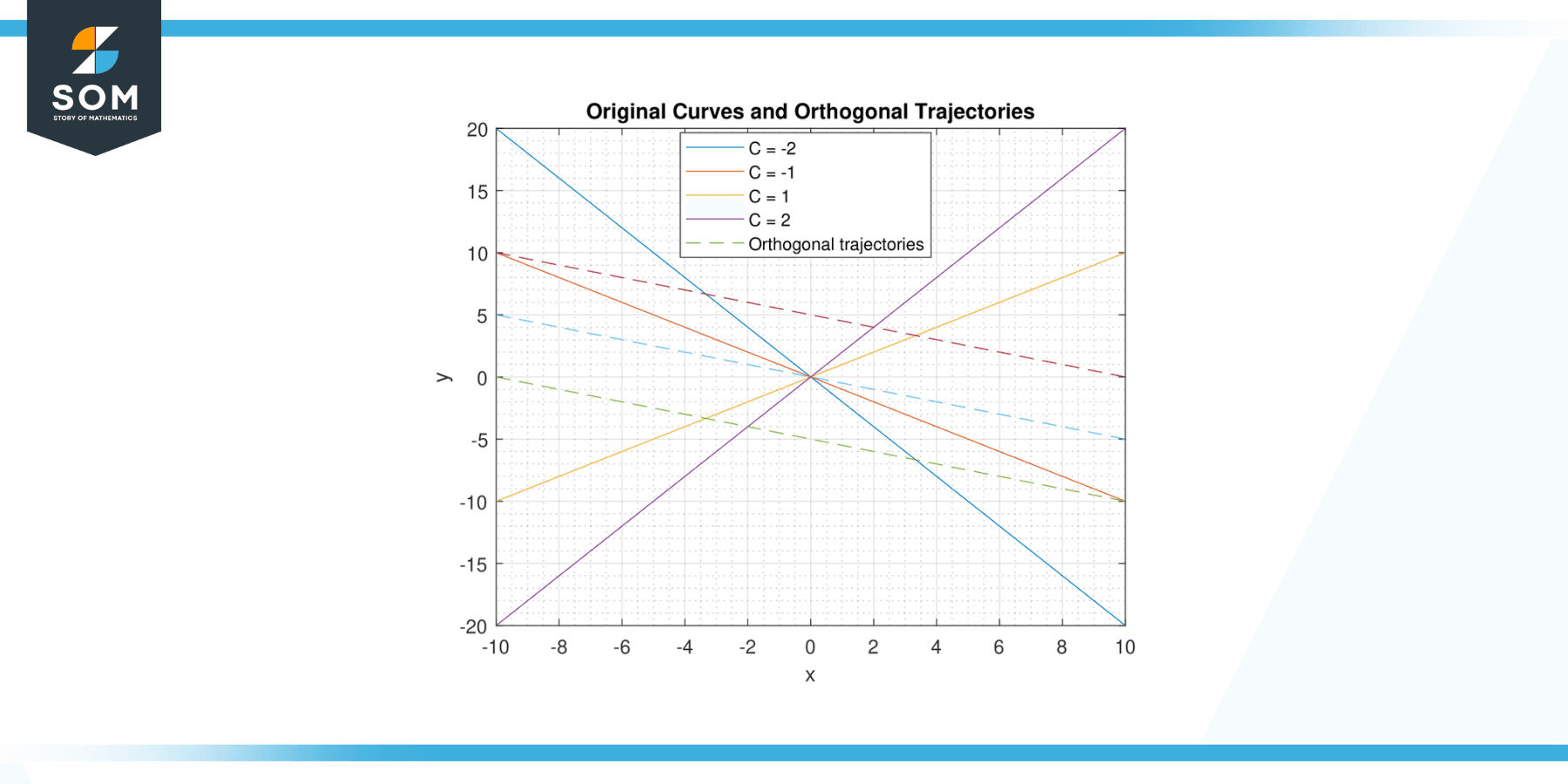
Figure-2.
Solution
For this, we need to take the derivative of y with respect to x. Doing so gives us:
dy/dx = C
The orthogonal trajectory will have a slope that is the negative reciprocal of this, or -1/C. We can then express this as a differential equation:
dy/dx = -1/C
Solving this differential equation gives us:
y = -x/C + D
where D is the constant of integration.
This is the family of curves that are orthogonal to the original family.
Example 2
Find the orthogonal trajectories of the family of curves defined by y = C/x, where C is a constant.
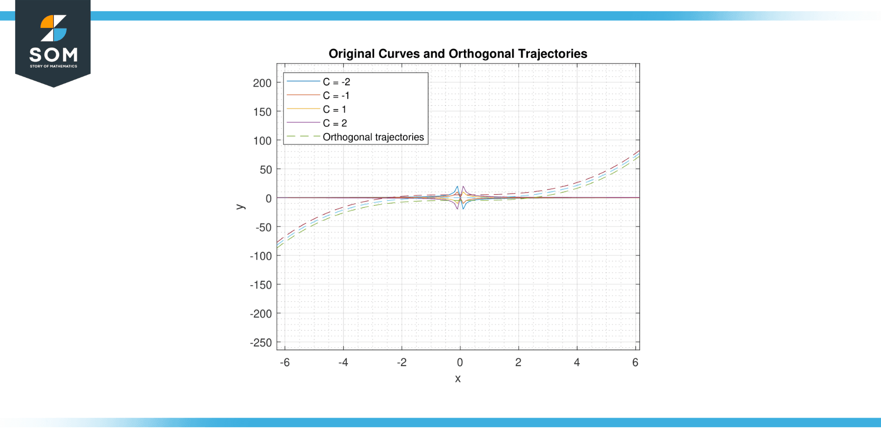
Figure-3.
Solution
First, compute dy/dx to get -C/x². The orthogonal trajectory will have a slope that is the negative reciprocal of this, or x²/C. This can be expressed as a differential equation:
dy/dx = x²/C
Solving this differential equation gives us:
y = (1/3C)x³ + D
where D is the constant of integration.
This is the family of curves that are orthogonal to the original family.
Example 3
Find the orthogonal trajectories of the family of curves defined by x² + y² = C.
Solution
Differentiating gives 2x + 2y(dy/dx) = 0. Simplifying gives:
dy/dx = -x/y
The orthogonal trajectory will have a slope that is the negative reciprocal of this, or y/x.
Expressing this as a differential equation gives:
dy/dx = y/x
Solving this differential equation by separating variables and integrating gives us:
y = Cx
where C is the constant of integration.
This is the family of curves that are orthogonal to the original family.
Example 4
Find the orthogonal trajectories of the family of curves y² - x² = C.
Solution
Differentiating gives:
2y(dy/dx) - 2x = 0
Simplifying gives:
dy/dx = x/y
The orthogonal trajectory will have a slope that is the negative reciprocal of this, or -y/x.
Expressing this as a differential equation gives:
dy/dx = -y/x
Solving this differential equation by separating variables and integrating gives us:
y = C/x
where C is the constant of integration.
This is the family of curves that are orthogonal to the original family.
All images were created with MATLAB.