JUMP TO TOPIC

In the vast and interconnected realm of mathematical functions, quartic functions hold a position of unique interest and versatility. Characterized by a degree of four, these functions, defined by a fourth-degree polynomial, wield significant influence across numerous aspects of mathematical theory and its many practical applications.
As the next step beyond linear, quadratic, and cubic functions, quartic functions offer higher complexity and potential for variability in their graphs.
This article explores quartic functions comprehensively, investigating their distinct features, mathematical properties, and far-reaching implications across diverse disciplines, including physics, engineering, and computer graphics.
Whether you’re a budding mathematician, an experienced scholar, or simply someone intrigued by the inherent beauty of mathematical patterns, this journey into the world of quartic functions promises to broaden your horizons.
Definition of the Quartic Function
A quartic function, also known as a biquadratic function or a polynomial of degree four, is a polynomial function with the highest degree being four. It can be generally expressed in the standard form as:
f(x) = ax⁴ + bx³ + cx² + dx + e
In this equation, ‘x’ represents the variable, and ‘a’, ‘b,’ ‘c,’ ‘d’, and ‘e’ are coefficients. ‘a’ is the leading coefficient, and it should not be equal to zero, because if ‘a’ were zero, the highest power of ‘x’ would be less than four, and the function would not be quartic function. Below we present two different generic quartic functions in Figure-1.
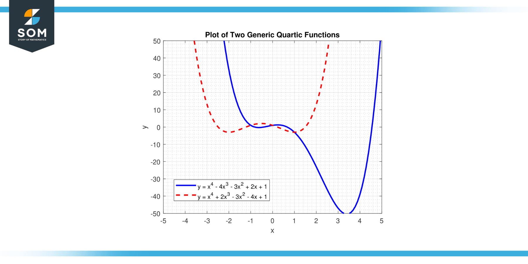
Figure-1.
The solutions to the equation f(x) = 0 are the roots of the quartic function, and it can have up to four roots, which may be real or complex numbers. The graph of a quartic function is called a quartic curve.
Depending on the values of the coefficients, the quartic curve can have various shapes, including a single curve with a single peak and trough, an “M” or “W” shaped curve with two peaks and a trough, or a curve resembling a cubic function with an additional loop.
The quartic function can model various real-world phenomena, making it a useful tool in various fields such as physics, engineering, computer graphics, and more. The study of quartic functions contributes significantly to understanding polynomial functions and their applications.
Graphical Analysis of Quartic Functions
As a polynomial of degree four, a quartic function has a diverse range of potential graph shapes. Here’s how to understand and analyze them:
General Shape
Quartic functions can have various general shapes depending on the coefficients in the equation. In particular, if the leading coefficient (the coefficient of the x⁴ term) is positive, the function opens upwards at both ends, while if it’s negative, it opens downwards. This is similar to the behavior of quadratic functions but with an additional level of complexity due to the higher degree. Below we present two different generic quartic functions in Figure-2. One opening upwards and one opening downwards.
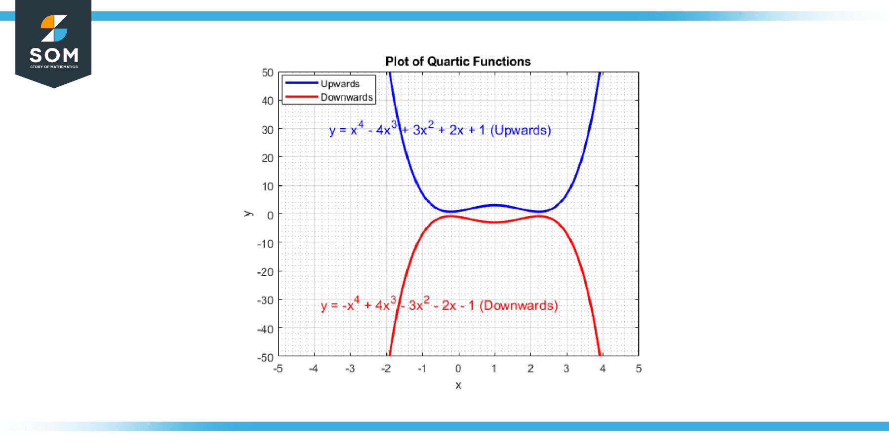
Figure-2.
The number of Turning Points
A quartic function can have up to three turning points, or local minima and maxima, where the function changes direction.
Extrema
A quartic function will have one or two local extrema (maximum or minimum points). This is determined by the coefficients of the function.
Inflection Points
Quartic functions can also have inflection points where the curvature of the function changes direction. A quartic function can have either one or two inflection points.
Symmetry
A quartic function can exhibit two types of symmetry. If all terms in the function have even powers, the graph will be symmetric about the y-axis. If all terms with nonzero coefficients are odd powers, the graph will be symmetric with respect to the origin.
Intercepts
The x-intercepts of the quartic function are the real roots of the corresponding polynomial equation, and the y-intercept is the constant term in the equation.
End Behavior
The end behavior of a quartic function resembles that of a quadratic function. If the leading coefficient is positive, the graph rises to positive infinity as x equals positive or negative infinity. If the leading coefficient is negative, the graph descends to negative infinity as x goes to positive or negative infinity.
In conclusion, with their potential for complex behavior, quartic functions offer an intriguing topic for graphical analysis. Through careful study of their key features, one can gain a deeper understanding of the nature and characteristics of these interesting functions.
Maximum and Minimum Points of a Quartic Function
Quartic functions are polynomial functions of degree four, and they can exhibit both local maximums and minimums, as well as a global maximum or minimum.
Local Maximum and Minimum Points
These are the points in the function where the curve changes direction from increasing to decreasing (for a local maximum) or decreasing to increasing (for a local minimum). They are called “local” because they represent the highest or lowest points within a certain interval or “neighborhood” around these points. Below we present the local maxima and local minima points of a generic quartic function in Figure-3.
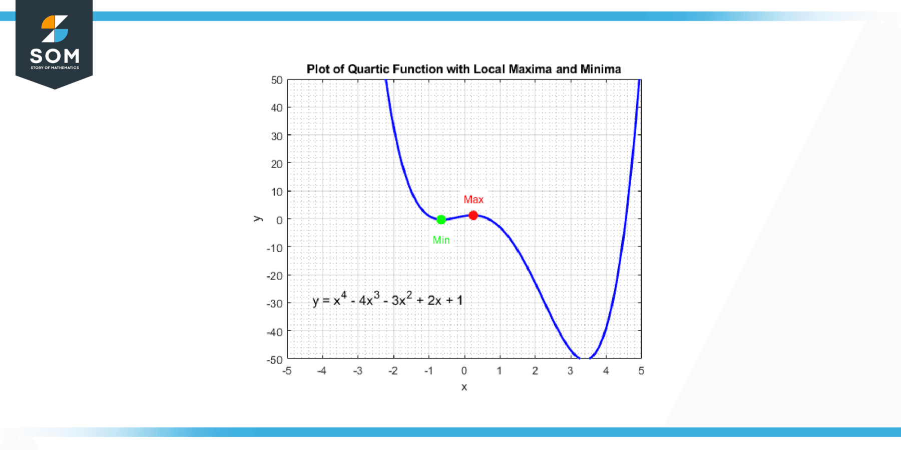
Figure-3.
Global Maximum and Minimum Points
These are the highest and lowest points over the entire function domain. For a quartic function, it’s possible that the global maximum or minimum might occur at the local maximum or minimum points. Still, it might also happen at the endpoints of the function (where the function is either rising or falling toward infinity).
You can find these points by taking the derivative of the quartic function, which will give you a cubic function. You then solve for the values of x that make the derivative equal to zero because these x-values correspond to the points where the quartic function has a local maximum, a local minimum, or a point of inflection. Below we present the global maxima point of a generic quartic function in Figure-4.
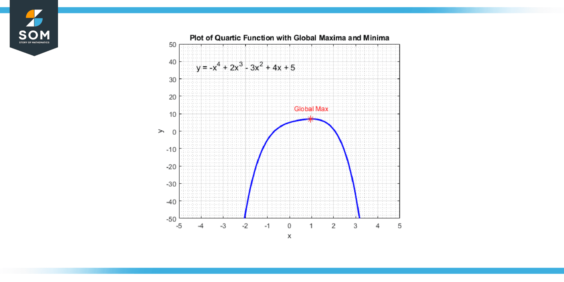
Figure-4.
Once you have these x-values, you can substitute them into the original quartic function to find the corresponding y-values. These (x, y) pairs are your local maxima and minima. Note that if the quartic function changes from increasing to decreasing at one of these points, you have a local maximum; if it changes from decreasing to increasing, you have a local minimum.
A quartic function’s global maximum and minimum can only occur at these local maximum and minimum points or the endpoints of the function’s domain. To find the global maximum and minimum, you compare the y-values of these points and the endpoints.
Note that the second derivative of the quartic function can be used to determine whether each critical point (where the first derivative equals zero) is a local maximum, local minimum, or point of inflection. If the second derivative at a critical point is negative, that point is a local maximum; if it’s positive, the point is a local minimum; if it’s zero, the second derivative test is inconclusive, and you need to use other methods to classify the critical point.
Solving Quartic Functions
Quartic equations are equations of the fourth degree, that is, equations that involve the variable x raised to the power 4. The general form of a quartic equation is:
ax⁴ + bx³ + cx² + dx + e = 0
Solving quartic equations can be done through various methods, the most general being Ferrari’s. However, this complex method requires a good understanding of algebraic manipulation. For most practical purposes, numerical methods or specialized software are used to solve quartic equations.
Here is a basic summary of the steps involved in Ferrari’s method:
Depress the Quartic
This step involves transforming the quartic equation into a depressed quartic equation, which doesn’t have a cubic term. This is done by substituting x = (y – b/4a) into the equation. The equation then takes the form: y⁴ + fy² + g = 0, where f and g are derived from a, b, c, d, and e.
Solve the Resolvent Cubic
The next step is to find a value p such that the equation y⁴ + fy² – (f²)/4 + g = 0 can be written as (y² + f/2 + p)² = 4p² – g. The value p satisfies the resolvent cubic equation: 8p³ + 4fp² + 8gp – f² = 0. This cubic equation can be solved using the cubic formula or other methods for solving cubic equations.
Find the Square Roots
Once the p-value is known, the original equation can be rewritten as (y² + f/2 + p + q)² = (2p – q)², where q is one of the square roots of 4p² – g. Solving for y² in this equation gives two possibilities: y² = -f/2 – p ± √((f/2 + p)² – g).
Solve for y
Finally, taking the square roots of the solutions for y² gives four solutions for y. Substituting y = x + b/4a back into these solutions gives the four solutions for x.
As mentioned, this method is rather complex and tedious to carry out by hand. More often than not, specialized mathematical software or calculators are used to solve quartic equations, especially when they are not easily factorable or do not have rational roots.
Note that some special cases of quartic equations can be solved more easily. For instance, if the quartic equation is biquadratic (i.e., of form ax⁴ + bx² + c = 0), it can be solved by first substituting y = x², reducing the equation to a quadratic equation in y, then solving for y and finally for x. Another special case is when the quartic equation can be factored into two quadratic equations, in which case the quadratic formula can be used to find the roots.
Applications
Quartic functions, which are polynomial functions of the fourth degree, have a variety of applications in different fields. Here are a few examples:
Physics
Quartic functions often appear in problems dealing with equilibrium, particularly in calculating potential energy. For example, the potential energy of a simple harmonic oscillator (like a mass attached to a spring) can be represented by a quartic function if the displacement of the mass from its equilibrium position is large. The quartic function also appears in the physics of liquid crystals, where the system’s potential energy can be expressed as a quartic function of the order parameter.
Engineering
Quartic equations often arise in engineering fields. For example, in mechanical engineering, the deflection of beams under load can lead to quartic equations. In civil engineering, a quartic function can model the shape of a suspension bridge cable under its own weight and the weight of a uniformly distributed load.
Computer Science & Computer Graphics
Quartic functions are used in Bezier curves and utilized in vector graphic applications and computer-aided design (CAD) software. A Bezier curve of degree 4 is determined by five points, and a quartic function describes the curve. This has implications in various fields such as animation, modeling of shapes, and in digital image processing.
Optics
In optics, quartic functions are used to model the wavefront aberrations caused by the variations in the thickness of a lens or a mirror.
Mathematical Problems & Games
Quartic functions can be used to solve certain types of mathematical puzzles and games. For instance, problems involving the intersection of circles and hyperbolas can lead to quartic equations. The peg solitaire game has been mathematically analyzed using quartic functions.
Finance
In finance, quartic functions can sometimes be used to model and predict trends in data that exhibit three turning points over a specific interval.
It’s important to note that while quartic functions can model many real-world phenomena, they’re not always the most practical or efficient tools for the job. Other functions or numerical methods might be more appropriate in many cases, depending on the specific problem and the available data.
Exercise
Example 1
Find the roots of the quartic equation: x⁴ – 5x² + 6 = 0
Solution
This is a biquadratic equation, so we can substitute y = x² and solve the resulting quadratic equation. We get:
y² – 5y + 6 = 0
Factoring this gives:
(y – 2)(y – 3) = 0
So, the solutions for y (the values of x²) are y = 2 and y = 3. Then, solving for x gives the four roots of the original quartic equation:
x = ±√(2), ±√(3)
Example 2
Consider the following equation: x⁴ – 13x² + 36 = 0, and find its roots.
Solution
Again, this is a biquadratic equation to substitute y = x². We then get:
y² – 13y + 36 = 0
This factors to:
(y – 4)(y – 9) = 0
So the solutions for y (the values of x²) are y = 4 and y = 9. Solving for x then gives the four roots of the original quartic equation:
x = ±2, ±3
Example 3
For the quartic function: f(x) = x⁴ – 6x² + 8, find the x-values at which the function has local maxima or minima.
Solution
Local maxima and minima occur where the derivative of the function is zero. So we first need to find the derivative of f:
f'(x) = 4x³ – 12x
Setting this equal to zero gives:
4x³ – 12x = 0
This can be factored to:
4x(x² – 3) = 0
Setting each factor equal to zero gives the solutions:
x = 0, ±√(3)
So the quartic function f(x) has local maxima or minima at x = 0 and x = ±√(3).
To determine whether these points are maxima or minima, we could use the second derivative test:
f”(x) = 12x² – 12
Evaluating the second derivative at each critical point, we find:
f”(0) = -12 (< 0, so x = 0 is a local maximum)
f”(-√(3)) = 24 – 12 = 12 (> 0, so x = –√(3) is a local minimum)
f”(√(3)) = 24 – 12 = 12 (> 0, so x = √(3) is a local minimum)
So, the function has a local maximum at x = 0 and local minima at x = –√(3) and x = √(3).
Example 4
Solve the quartic equation: x⁴ – 2x³ – 8x² + 16x = 0
Solution
This equation can be factored by grouping:
x(x³ – 2x² – 8x + 16) = 0
And then factor the cubic term:
x(x – 2)(x² + 4) = 0
The solutions are then:
x = 0, 2, ±2i
So this quartic equation has two real roots (0 and 2) and two complex roots (±2i).
Example 5
Find the critical points of the quartic function: f(x) = x⁴ – 4x³ + 6x² – 4x + 1
Solution
Critical points occur where the derivative of the function is zero. So we first need to find the derivative of f:
f'(x) = 4x³ – 12x² + 12x – 4
Setting this equal to zero gives:
4x³ – 12x² + 12x – 4 = 0
This can be factored as:
4(x – 1)³ = 0
Setting the factor equal to zero gives the solution:
x = 1
So, the quartic function f(x) has one critical point at x = 1. To determine whether this point is a maximum, minimum, or inflection point, we could use the second derivative test:
f”(x) = 12x²– 24x + 12
Evaluating the second derivative at the critical point, we find:
f”(1) = 12 – 24 + 12 = 0
Since the second derivative equals zero, the second derivative test is inconclusive. We could determine the nature of the critical point by looking at the sign of the first derivative to the left and right of x = 1 or by considering higher-order derivatives. Still, either of these approaches would involve further work.
Example 6
Find the roots of the quartic equation: x⁴ – 2x³ – 13x² + 14x + 24 = 0
Solution
This is a non-trivial quartic equation and can’t be easily factored or solved by substitution. However, you can solve it numerically with software like Wolfram Alpha or a calculator that can handle complex roots. When you do this, you find that the quartic has two real roots and two complex roots:
x ≈ 3.64575, -0.645753, 0.5 – 2.17945i, 0.5 + 2.17945i
So this quartic equation has two real roots and two complex roots.
All images were created with GeoGebra and MATLAB.