JUMP TO TOPIC
Sampling variability focuses on how well-dispersed a given set of data is. When dealing with real-world data or large-scale surveys, it is nearly impossible to manipulate the values one by one. This is when the concept of the sample set and sample mean enter – conclusions will depend on the measures returned by a sample set.
Sampling variability uses sample mean and the standard deviation of the sample mean to show how spread out the data are.
This article covers the fundamentals of sampling variability as well as the key statistical measures used to describe variability among a given sample. Learn how the standard deviation of a sample mean is calculated and understand how to interpret these measures.
What Is Sampling Variability?
Sampling variability is a range that reflects how close or far a given sample’s “truth” is from the population. It measures the difference between the sample’s statistics and what the population’s measure reflects. This highlights the fact that depending on the selected sample, the mean changes (or varies).
The sampling variability is always represented by a key statistical measure including the variance and standard deviation of the data. Before diving into the technical techniques of sampling variability, take a look at the chart shown below.
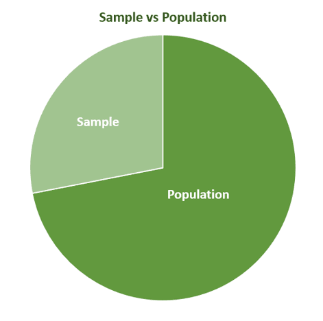
As can be seen, the sample only represents a portion of the population, showing how important it is to take note of the sampling variability. The chart also illustrates how in real-world data, the sample size may not be perfect but the best one highlights the closest estimate reflecting the population’s value.
Suppose that Kevin, a marine biologist, needs to estimate the weight of the shells existing near the seashore. His team has collected $600$ shells. They know that it will take time to weigh each shell, so they decide to use the mean weight of $240$ samples to estimate the weight of the entire population.
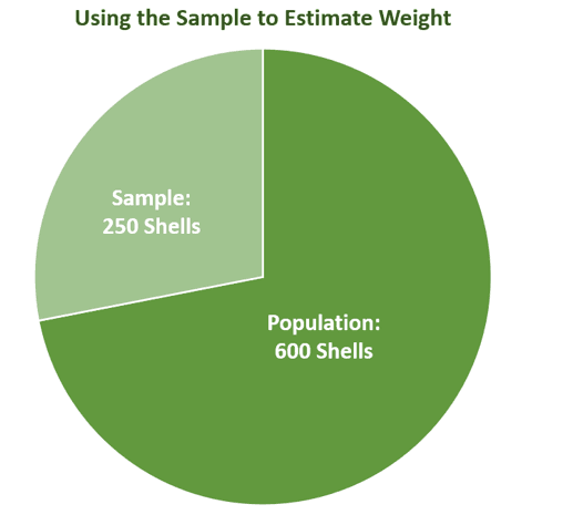
Imagine selecting $240$ shells from a population of $600$ shells. The mean weight of the sample will depend on the shells that were weighed — confirming the fact that the mean weight will vary depending on the sample size and the sample instead. As expected, if the sample size (how large a sample is) increases or decreases, the measures reflecting sampling variability will also change.
For accuracy’s sake, Kevin’s team weighed $240$ randomly-selected shells three times to observe how the sample’s mean weight varies. The diagram below summarizes the result of the three trials.
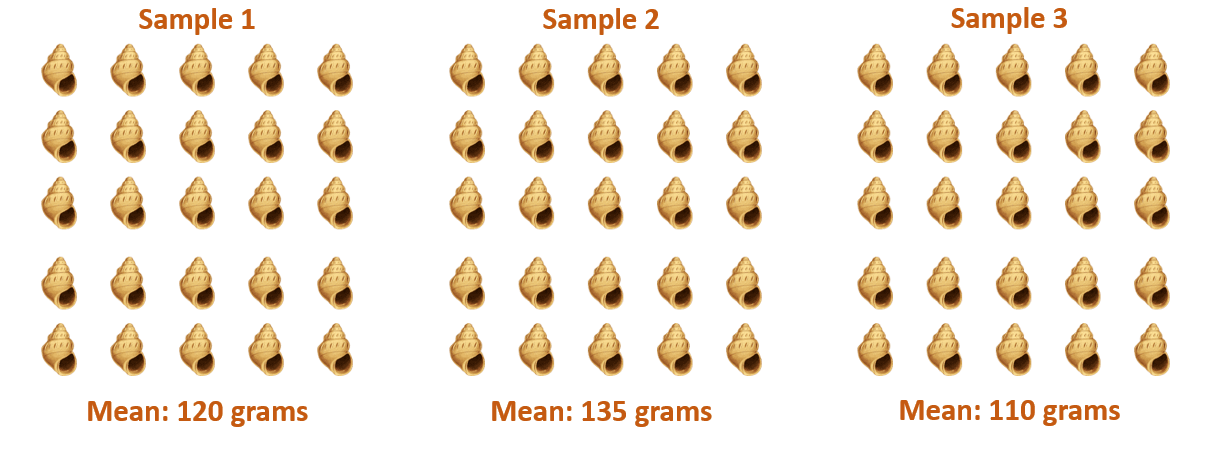
One shell represents $10$ shells, so each sample mean was calculated by weighing $250$ shells each. The three samples’ results shows varying mean weight: $120$ grams, $135$ grams, and $110$ grams.
This highlights the variability present when working with sample sizes. When working with only one sample or trial, the measures of sampling variability must be accounted for.
What Are Sampling Variability Measures?
The important measures used to reflect sampling variability are the sample’s mean and the standard deviation. The sample mean ($\overline{x}$) reflects the variation between the resulting means from the selected sample and consequently, the sampling variability of the data. Meanwhile, the standard deviation ($\sigma$) shows how “spread out” the data is from each other, so it also highlights the sampling variability in a given data.
- Calculating one sample mean ($\mu_\overline{x}$) saves time as opposed to calculating the entire population mean ($\mu$).
\begin{aligned}\mu =\mu_{\overline{x}}\end{aligned}
- Find the standard deviation of the sample mean ($\sigma_{\overline{x}}$)to quantify the variability present within the data.
\begin{aligned}\sigma_{\overline{x}} &=\dfrac{\sigma}{\sqrt{n}}\end{aligned}
Going back to the shells from the previous section, suppose that Kevin’s team only weighed one set of samples composed of $100$ shells. The calculated sample mean and standard deviation will then be as shown:
\begin{aligned}\textbf{Sample Size} &:100\\\textbf{Sample Mean} &: 125 \text{ grams}\\\textbf{Standard Deviation} &:12\text{ grams}\end{aligned}
To calculate the standard deviation of the sample mean, divide the given standard deviation by the number of shells (or the sample size).
\begin{aligned}\sigma_{\overline{x}} &=\dfrac{12 }{\sqrt{100}}\\ &= 1.20 \end{aligned}
This means that although the best estimate of the average weight of all $600$ shells is $125$ grams, the average weight of the shells from the selected sample will vary by approximately $1.20$ grams. Now, observe what happens when the sample size increases.
What if Kevin’s team got the sample mean and standard deviation with the following sample sizes?
Sample Size | Standard Deviation of the Sample Mean |
\begin{aligned}n =150\end{aligned} | \begin{aligned}\sigma_{\overline{x}} &= \dfrac{12 }{\sqrt{150}}\\&= 0.98 \end{aligned} |
\begin{aligned}n =200\end{aligned} | \begin{aligned}\sigma_{\overline{x}} &= \dfrac{12 }{\sqrt{200}}\\&= 0.85 \end{aligned} |
\begin{aligned}n =250\end{aligned} | \begin{aligned}\sigma_{\overline{x}} &= \dfrac{12 }{\sqrt{200}}\\&= 0.76 \end{aligned} |
As the sample size increases, the sample mean’s standard decreases. This behavior makes sense, since the larger the sample size, the smaller the difference between the sample mean measured.
The next section will show more examples and practice problems highlighting the significance of the sampling variability measures that have been discussed.
Example 1
A dormitory has been planning to implement new curfew hours and the dormitory administrator claims that $75\%$ of the residents are in support of the policy. There are some residents, however, that want to review the data and the administrator’s claim.
To refute this claim, the residents organized a survey of their own where they randomly ask $60$ residents whether they are in favor of the new curfew hours. From the $60$ residents asked, $36$ residents are okay with the proposed curfew hours.
a. This time, how many percent were in favor of the new proposed curfew hours?
b. Compare the two values and interpret the difference in percentage.
c. What can be done so that the residents will have better claims and be able to refute the proposed curfew hours?
Solution
First, find the percentage by dividing $36$ by the total number of residents asked ($60$) and multiply the ratio by $100\%$.
\begin{aligned}\dfrac{36}{60} \times 100\% &= 60\%\end{aligned}
a. This means that after performing their survey, the residents found out that only $60\%$ were in favor of the proposed curfew hours.
A survey by the Dorm Administrator | \begin{aligned}75\%\end{aligned} |
Survey by Residents | \begin{aligned}60\%\end{aligned} |
b. From these two values, the residents have found fewer students in favor of the new curfew hours. The $15\%$ difference can be the result of residents having encountered more residents against the curfew hours.
If they randomly selected more residents in favor of the curfew hours, these percent differences may shift in favor of the dormitory administrator. This is due to the sampling variability.
c. Since sampling variability has to be accounted for, the residents should tweak their process to provide more concrete claims to reject the proposal by the dormitory administrator.
Since standard deviation decreases by increasing the sample size, they can ask more residents for a better overview of the entire population’s opinion. They should set a reasonable number of respondents based on the total number of residents in the dormitory.
Example 2
The moderators of a book enthusiast virtual community held a survey and asked their members the number of books they read in a year. The population mean shows an average of $24$ books with a standard deviation of $6$ books.
a. If a subgroup with $50$ members was asked the same question, what is the mean number of books read by each member? What will the calculated standard deviation be?
b. What happens with the standard deviation when a larger subgroup with $80$ members is asked?
Solution
The sample mean will be equal to the given population mean, so the first subgroup would have read $24$ books. Now, use the sample size to calculate the standard deviation for $50$ members.
\begin{aligned}\sigma_{\overline{x}} &=\dfrac{6}{\sqrt{50}}\\ &=0.85 \end{aligned}
a. The sample mean for the subgroup remains the same: $24$, while the standard deviation becomes $0.85$.
Similarly, the sample mean for the second subgroup is still $24$ books. However, with a larger sample size, the standard size is expected to decrease.
\begin{aligned}\sigma_{\overline{x}} &=\dfrac{6}{\sqrt{80}}\\&= 0.67 \end{aligned}
b. Hence, the sample mean is still $24$ but the standard deviation has further decreased to $0.67$.
Practice Questions
1. True or False: The sample mean becomes smaller as the sample size increases.
2. True or False: The standard deviation reflects how spread out the sample mean is for each sample set.
3. A random sample with a size of $200$ has a population mean of $140$ and a standard deviation of $20$. What is the sample mean?
A. $70$
B. $140$
C. $200$
D. $350$
4. Using the same information, by how much will the standard deviation of the sample mean increase or decrease if the sample size is now $100$?
A. The standard deviation will increase by a factor of $\sqrt{2}$.
B. The standard deviation will increase by a factor of $2$.
C. The standard deviation will decrease by a factor of $\sqrt{2}$.
D. The standard deviation will increase by a factor of $\dfrac{1}{2}$.
Answer Key
1. False
2. True
3. C
4. A