Uniform Continuity – Definition and Examples

This article aims to delve into the labyrinth of uniform continuity, illuminating its distinct attributes, elucidating its relevance in the world of mathematics, and demystifying its application in practical scenarios.

Defining Uniform Continuity

Uniform Contuinity is a property of a coreesponding mathematical function. In mathematical analysis, a function is said to be uniformly continuous if, roughly speaking, it is possible to guarantee that the outputs of the function are as close together as we want for all sufficiently close inputs, irrespective of where in the domain these inputs are located.

More formally, a function ‘f’ defined on a set ‘S’ is uniformly continuous if for every positive number ε (no matter how small), there exists a positive number δ such that for every pair of points ‘x’ and ‘y’ in ‘S’, if the distance between ‘x’ and ‘y’ (|x-y|) is less than δ, then the distance between f(x) and f(y) (|f(x)-f(y)|) is less than ε.

This is a stronger condition than ordinary continuity, which requires this property to hold only for sufficiently close points ‘x’ and ‘y’ in a small interval around each point in the domain. The notion of uniform continuity, however, requires the function to exhibit this property simultaneously for all points in its domain.

Example

Prove that the function f(x) = √x is uniformly continuous on the interval [0, ∞).

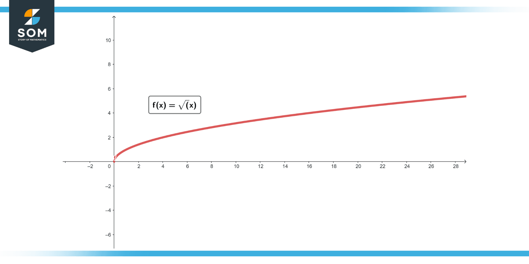
Figure-1.

Solution

By the definition of uniform continuity, for every ε > 0, we must find a δ > 0 such that for all x, y in the domain, if |x – y| < δ, then |f(x) – f(y)| < ε.

Choose an arbitrary ε > 0

First we choose an arbitrary value for ε.

Try to Express δ in Terms of Ε ε

We want to show that if |x – y| < δ, then |f(x) – f(y)| < ε, or |√x – √y| < ε.

To make this easier, we can square both sides of the latter inequality (since both sides are nonnegative), giving:

|x – y| < ε²

So, if we take δ = ε², then |x – y| < δ implies |x – y| < ε².

Check that |f(x) – f(y)| < ε when |x – y| < δ

From the previous step, we know that |x – y| < ε². Now, we consider |f(x) – f(y)|, which is:

|√x – √y|

Notice that (|√x – √y|)² = |x – y|, which is less than ε², so |√x – √y| < ε, which is exactly what we wanted to show.

So, for every ε > 0, we found a corresponding δ (in this case, δ = ε²) such that whenever |x – y| < δ, we have |f(x) – f(y)| < ε, for all x, y in the interval [0, ∞).

Hence, f(x) = √x is uniformly continuous on [0, ∞).

Uniform Contuinity Theorem

A function that is continuous on a closed interval [a, b] is uniformly continuous on that interval.

Proof

We will prove this by contradiction. Suppose f is a function that is continuous on [a, b] but not uniformly continuous.

That means there exists an ε > 0 such that for every δ > 0, there exist points x, y in [a, b] with |x – y| < δ and yet |f(x) – f(y)| ≥ ε.

We can construct two sequences {xₙ} and {yₙ} in [a, b] such that |xₙ – yₙ| < 1/n for every natural number n, and yet |f(xₙ) – f(yₙ)| ≥ ε.

Since [a, b] is a compact set (it is closed and bounded), there exist subsequences {xₙₖ} and {yₙₖ} that converge to limits in [a, b], say x and y, respectively.

By the squeeze theorem, x = y.

Since f is continuous at x, given any ε > 0, there exists a δ > 0 such that whenever |x – t| < δ, |f(x) – f(t)| < ε.

Take K so large that 1/ₙₖ < δ for all k > K. Then when k > K, |xₙₖ – yₙₖ| < δ, so |f(xₙₖ) – f(yₙₖ)| < ε, contradicting the choice of the sequences.

Therefore, our assumption that f was not uniformly continuous is false, which means that f must be uniformly continuous.

So, any function continuous on a closed interval [a, b] is uniformly continuous on that interval.

Uniform Contuinity Evaluation Process

Evaluating whether a function is uniformly continuous requires applying the mathematical definition of uniform continuity, which states: A function f defined on a set S is said to be uniformly continuous if for any number ε > 0, there is a number δ > 0 such that for all x and y in S, if |x – y| < δ, then |f(x) – f(y)| < ε.

Here’s a step-by-step process of evaluating uniform continuity:

Understand the Function and Its Domain

You must first understand the function that you’re working with and the domain over which it is defined. Uniform continuity applies to the entire domain of the function.

Choose Arbitrary ε > 0

For a function to be uniformly continuous, it needs to hold true for any ε greater than 0, so it is usually easier to start by letting ε be an arbitrary positive number.

Find δ in Terms of ε

The hardest part of the process usually involves finding a δ > 0 such that if |x – y| < δ for any x, y in the domain, then |f(x) – f(y)| < ε. This step often involves manipulating the inequality |f(x) – f(y)| < ε to solve for δ.

Check That the Condition Holds for All X, Y in the Domain

Once you have found a possible δ, you should verify that the condition of uniform continuity holds for all pairs of points in the domain of the function.

Use Theorems When Applicable

If the function is continuous and the domain is a closed and bounded interval (i.e., a closed interval [a, b] in the real numbers), then the function is uniformly continuous by the Heine-Cantor theorem. You can use this theorem to quickly establish uniform continuity for functions on closed intervals.

If at any point in the process you find that there is no δ that satisfies the condition for every pair of points x, y in the domain, then the function is not uniformly continuous. Conversely, if you can find such a δ for any given ε > 0, then the function is uniformly continuous.

Remember, the key feature of uniform continuity is that the δ does not depend on the choice of x or y in the domain, but only on ε. If your δ is dependent on x or y, then your function is not uniformly continuous.

Properties of Uniform Continuity

Uniform continuity shares many of the properties of ordinary continuity, but it has some unique ones that make it a more robust and powerful concept. Here are the most important properties of uniform continuity:

Preservation Under Limits

If a sequence of uniformly continuous functions{$f_n$} on a set S converges uniformly to a function f on S, then the limit function f is also uniformly continuous.

Preservation Under Composition

The composition of two uniformly continuous functions is uniformly continuous. If f: X → Y and g: Y → Z are two uniformly continuous functions, then their composition g∘f: X → Z is also uniformly continuous.

Restrictions and Extensions

If a function is uniformly continuous on a set S, then it is uniformly continuous on any subset of S. Conversely, if a function is uniformly continuous on a set S and is extended to a larger set where it is continuous, it remains uniformly continuous on S.

Boundedness on Compact Sets

If a function is uniformly continuous on a compact set (in a metric space), it is also bounded on that set.

Lipschitz Condition

A uniformly continuous function on a closed interval [a, b] satisfies the Lipschitz condition, i.e., there exists a constant L such that for all x, y in [a, b], |f(x) – f(y)| ≤ L|x – y|. This means that the function does not exhibit “extreme behavior”, such as infinite slopes or asymptotic behaviors within the interval.

Continuous Images of Compact Sets

If a function is uniformly continuous on a set S, and K is a compact subset of S, then f(K) is also compact. This is a consequence of the Heine-Cantor theorem which states that a continuous function on a compact set is uniformly continuous.

Uniform Continuity and Sequences

A function f is uniformly continuous on a set S if and only if for every sequence ($x_n$), ($y_n$) in S that satisfies |$x_n – y_n$| → 0 as n → ∞, we have |f(x_n) – f(y_n)| → 0 as n → ∞.

Extension to Completion

Every uniformly continuous function from a dense subset of a metric space to another metric space can be uniquely extended to a uniformly continuous function on the whole space.

Remember that while all uniformly continuous functions are continuous, the reverse is not true. Regular continuity only considers points close to a specific point, while uniform continuity deals with points close anywhere in the domain. This distinction makes uniform continuity a stronger condition.

Ralevent Mathematics

The definition of uniform continuity relies more on the qualitative behavior of a function rather than specific formulas. However, there are a few mathematical expressions that are used to define and understand uniform continuity.

The formal definition of uniform continuity involves an epsilon-delta relation:

A function f defined on a set S in the real numbers is uniformly continuous if for all ε > 0, there exists a δ > 0 such that for all x, y in S, if |x – y| < δ, then |f(x) – f(y)| < ε.

The ε (epsilon) and δ (delta) are small positive numbers, and the inequality |x – y| < δ indicates that x and y are very close together, while |f(x) – f(y)| < ε expresses that the corresponding outputs f(x) and f(y) are also close together.

The key feature of uniform continuity is that the same δ value works for all x, y in S, meaning it doesn’t depend on the specific points chosen in the domain. This is in contrast to ordinary continuity, where δ might vary depending on the point x.

Regarding the Lipschitz condition, it is another specific condition related to uniform continuity. A function f(x) satisfies the Lipschitz condition on a set S if there exists a constant K > 0 such that for all x, y in S, |f(x) – f(y)| ≤ K |x – y|.

In other words, the rate at which the function changes (given by |f(x) – f(y)|) is bounded by a constant K times the distance between the points (|x – y|). Functions that satisfy the Lipschitz condition are uniformly continuous, but not all uniformly continuous functions satisfy the Lipschitz condition.

A function f is said to satisfy the Lipschitz condition if there exists a positive constant L such that for all x, y in the domain of f, |f(x) – f(y)| ≤ L|x – y|.

The constant L here is known as the Lipschitz constant. If a function satisfies the Lipschitz condition, it is uniformly continuous.

Both of these expressions encapsulate the idea of uniform continuity – the ability to bound the change in the function’s output by a constant times the change in the input, no matter where we are in the function’s domain. It’s important to remember that these are not “formulas” in the sense of something like the quadratic formula, but rather, they are definitions or conditions describing a certain type of behavior that a function might exhibit.

Exercise 

Example 1

The function f(x) = x² on the interval [0, 1] is uniformly continuous.

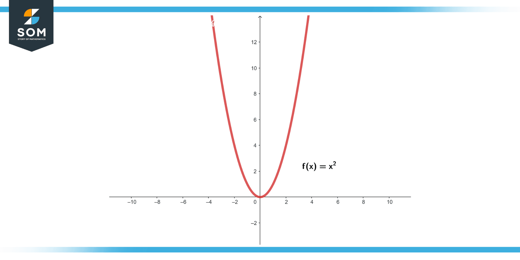
Figure-2.

Solution

To prove this, note that for any ε > 0, we can choose δ = √(ε/2) + 1.

Then, for any x, y ∈ [0, 1] with |x – y| < δ, we have:

|f(x) – f(y)| = |x² – y²|

|f(x) – f(y)| = |x – y||x + y|

|f(x) – f(y)| ≤ |x – y|(1 + 1)

|f(x) – f(y)| = 2|x – y| < 2 * δ

|f(x) – f(y)|= ε

Example 2

The function f(x) = x³ is uniformly continuous on the whole real line.

Solution

To prove this, note that for any ε > 0, we can choose $δ = (ε/3)^{(1/3)}$. Then, for any x, y ∈ ℝ with |x – y| < δ, we have:

|f(x) – f(y)| = |x³ – y³|

|f(x) – f(y)| = |x – y||x² + xy + y²|

|f(x) – f(y)|  ≤ |x – y|(x² + |xy| + y²)

|f(x) – f(y)| < δ³ + 3 * δ² + 3 * δ

|f(x) – f(y)|= ε

Example 3

The function f(x) = sin(x) is uniformly continuous on the whole real line.

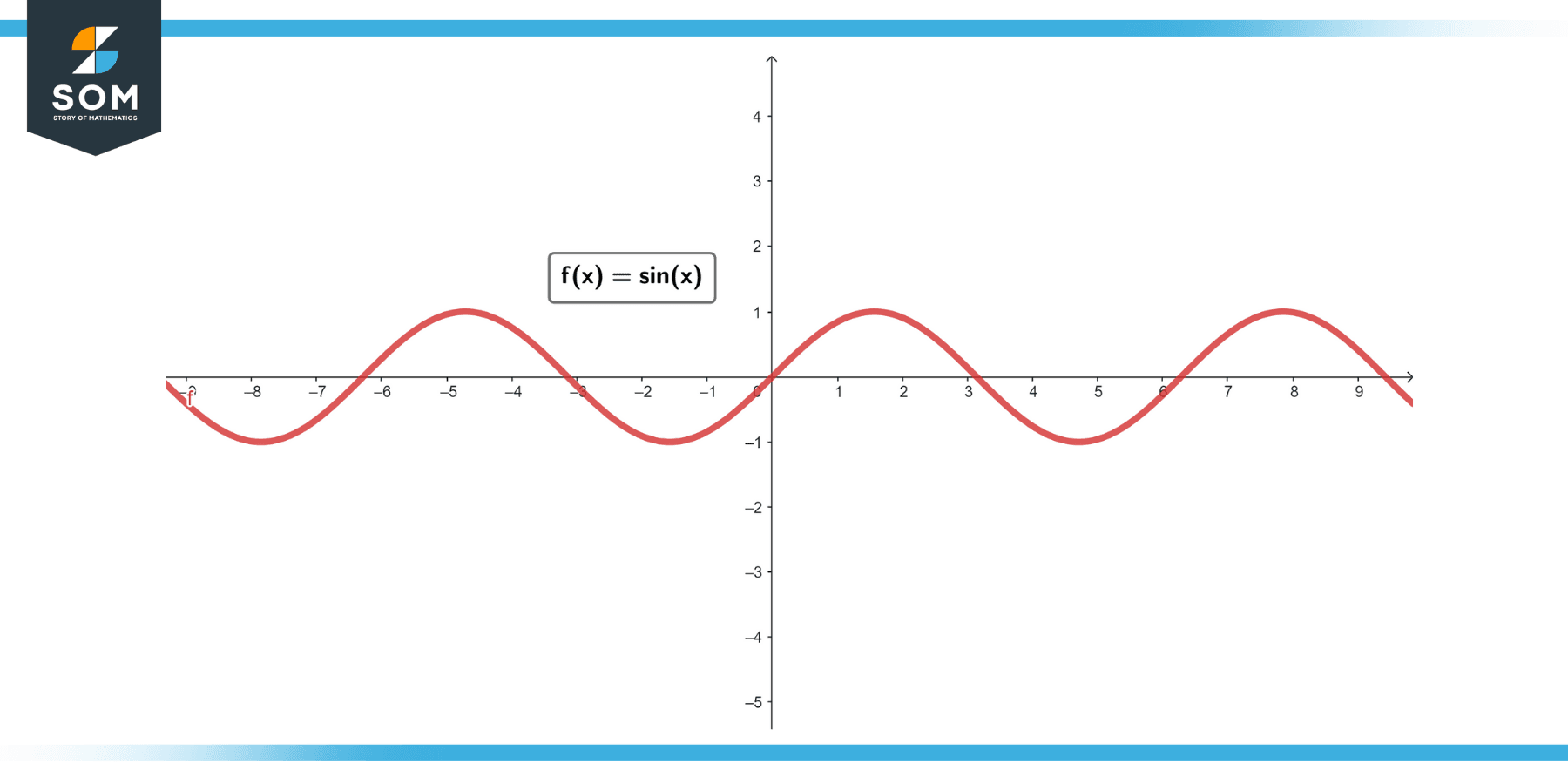
Figure-3.

Solution

To prove this, note that for any ε > 0, we can choose δ = ε. Then, for any x, y ∈ ℝ with |x – y| < δ, we have:

|f(x) – f(y)| = |sin(x) – sin(y)|

|f(x) – f(y)| ≤ |x – y|

|f(x) – f(y)| = δ

|f(x) – f(y)|= ε

Example 4

The function f(x) = √x is uniformly continuous on the interval [0, ∞).

Solution:

To prove this, note that for any ε > 0, we can choose δ = ε². Then, for any x, y ∈ [0, ∞) with |x – y| < δ, we have:

|f(x) – f(y)|

|f(x) – f(y)| = |√x – √y|

|f(x) – f(y)| ≤ √(|x – y|)

|f(x) – f(y)| = √(δ)

|f(x) – f(y)| = ε

Example 5

The function f(x) = 1/x is not uniformly continuous on the interval (0, ∞).

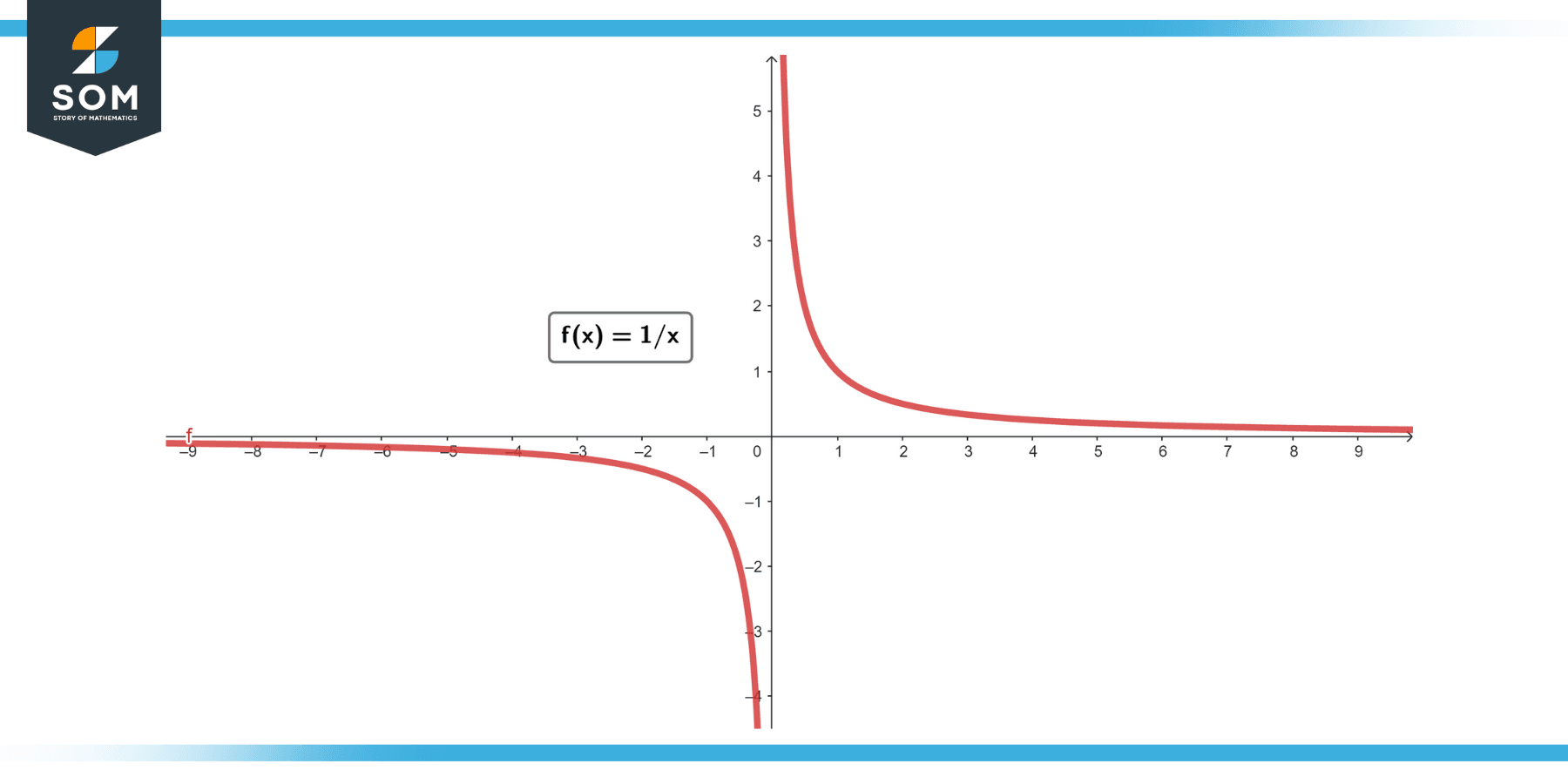
Figure-4.

Solution

To disprove this, suppose by contradiction that f is uniformly continuous.

Then, for ε = 1, there exists a δ > 0 such that if |x – y| < δ for x, y ∈ (0, ∞), then |1/x – 1/y| < 1. Take x = 1/2 and y = 1/(2 + δ). Then:

|x – y| < δ

but

|1/x – 1/y| = |2 – (2 + δ)| = δ

which contradicts our assumption.

Example 6

The function f(x) = eˣ is not uniformly continuous on the interval (-∞, ∞).

Solution

To disprove this, we consider two sequences: xₙ = n and yₙ = n + 1/n for n = 1, 2, …. Then:

|xₙ – yₙ| = 1/n goes to 0

but:

|f(xₙ) – f(yₙ)| = |eⁿ – eⁿ⁺¹⁄ₙ|

|f(xₙ) – f(yₙ)| = eⁿ * (e¹⁄ₙ – 1)

which does not go to 0.

Example 7

The function f(x) = ln(x) is uniformly continuous on the interval (0, ∞).

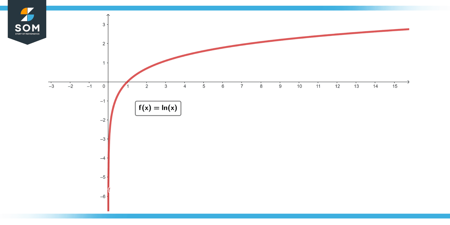
Figure-5.

Solution

To prove this, note that for any ε > 0, we can choose δ = eᵋ – 1. Then, for any x, y ∈ (0, ∞) with |x – y| < δ, we have:

|f(x) – f(y)| = |ln(x) – ln(y)|

|f(x) – f(y)| = |ln(x/y)|

|f(x) – f(y)| < ln(1 + δ)

|f(x) – f(y)| = ε

Example 8

Solution

The function f(x) = x² is not uniformly continuous on the whole real line.

To disprove this, we consider two sequences:

xₙ = n

and

yₙ = n + 1/n for n = 1, 2, ….

Then:

|xₙ – yₙ| = 1/n goes to 0

but:

|f(xₙ) – f(yₙ)| = |n² – (n + 1/n)²|

|f(xₙ) – f(yₙ)| = 2 * n * (1/n) + (1/n)²

|f(xₙ) – f(yₙ)| = 2 + 1/n

which does not go to 0.

Applications of Uniform Continuity

Uniform continuity, although a concept deeply rooted in pure mathematics, particularly in analysis and topology, has significant implications in numerous applications across various fields, including physics, engineering, computer science, and economics. Here are a few examples:

Physics

In physical models, uniform continuity often arises in context of ensuring the solution of differential equations used to model physical phenomena are well-behaved over specific intervals. For instance, the solution to a heat conduction or wave propagation problem must not only be continuous, but uniformly so to avoid abrupt changes.

Engineering

In control systems engineering, understanding uniform continuity is crucial for the stability analysis of systems. A bounded input leading to a bounded output (BIBO stability) often hinges on the assumption of uniform continuity of the system’s transfer function.

Computer Science

In the field of computer graphics and image processing, uniform continuity comes into play when dealing with transformations and mappings for textures, shapes, and surfaces. It ensures the graphical representation remains coherent and avoids sudden changes.

Economics and Finance

In mathematical economics and financial mathematics, the concept of uniform continuity is used to ensure the stability and smoothness of certain mathematical models. It can be applied in the context of modeling consumer behavior, market equilibria, and financial derivatives pricing, where continuous and predictable changes are assumed.

Numerical Analysis

Uniform continuity plays a crucial role in the approximation of functions using interpolating polynomials, ensuring that the error does not grow too large.

Probability Theory

Uniform continuity is used in the proof of fundamental theorems like the Kolmogorov Extension Theorem, which underlies the construction of stochastic processes.

Machine Learning and Artificial Intelligence

In certain aspects of machine learning and AI, such as neural networks and other function approximation methods, the underlying mathematics often relies on concepts like uniform continuity to ensure the “smoothness” and “learnability” of models.

Differential Geometry and Topology

Uniform continuity is a key concept in proving many results in these fields, such as embedding theorems, and plays a significant role in the understanding of manifold theory.

Function Approximation

In numerical analysis and approximation theory, uniformly continuous functions are critical because they allow us to make global approximations. If a function is uniformly continuous on an interval, then given any amount of error ε, there’s a step size (or resolution) δ such that any two points within that step size have function values within the desired error. This is used, for example, in numerical methods for solving differential equations.

Interchanging Limits

Uniform continuity is often used to justify the interchanging of limits, which is a common technique in mathematical analysis. For example, it allows one to interchange the order of integration and summation in a series of functions.

Ensuring Extendability of Functions

Uniformly continuous functions defined on a dense subset of a metric space can be uniquely extended to the entire space. This result, known as the extension theorem, has implications in areas of mathematics such as harmonic analysis.

Lipschitz Continuity

Uniform continuity is related to Lipschitz continuity, which is a stronger form of uniform continuity that arises in various fields. For example, the solutions to certain differential equations are Lipschitz continuous, which leads to their unique solvability.

Functional Analysis and Operator Theory

In functional analysis and operator theory, uniform continuity is a fundamental concept used in defining and studying different types of operators between Banach spaces.

Integration Theory

Uniform continuity is used in integration theory. For instance, a uniformly continuous function on a compact interval is Riemann integrable.

Fixed Point Theorems

Some fixed-point theorems, such as the Banach fixed-point theorem, require a form of uniform continuity (in this case, Lipschitz continuity) in their hypotheses.

It’s worth noting that while uniform continuity is an important concept, its applicability may not always be explicitly visible. Often, it is nested within broader mathematical tools or theorems used in these fields.

Historical Significance of Uniform Contuinity

Uniform continuity is a concept that arose from the formalization of analysis, a branch of mathematics, in the 19th century. As the foundations of calculus, originally developed by Sir Isaac Newton and Gottfried Wilhelm Leibniz in the 17th century, were being rigorously formulated, the notions of limits and continuity became more precise and better understood.

While Newton and Leibniz had relied on intuitive ideas of “infinitesimally small” quantities, mathematicians in the 19th century sought to eliminate these ambiguities. The result was a period of vigorous development in analysis, where mathematical giants like Karl Weierstrass, Augustin-Louis Cauchy, and Bernhard Riemann played pivotal roles.

The concept of uniform continuity, as a stronger version of continuity, emerged from these efforts. The term “uniform” refers to the fact that a uniformly continuous function preserves closeness uniformly throughout its domain. This is in contrast to ordinary continuity, which only ensures that closeness is preserved at individual points.

A key figure in these developments was Karl Weierstrass, a German mathematician. He introduced the “ε-δ” definition of limits and continuity, which set the stage for a precise understanding of these concepts. Weierstrass’s formalization provided the ground for defining uniform continuity in a rigorous way.

The introduction of uniform continuity had significant implications for analysis. For example, it led to the theorem that a continuous function on a closed interval is uniformly continuous, an important result in real analysis. It also played a critical role in the development of other branches of mathematics, such as functional analysis, measure theory, and topology.

The concept of uniform continuity continues to be a fundamental part of modern mathematical analysis and its various subfields. It’s an essential tool for understanding the properties of functions, spaces, and transformations in a rigorous way.

All images were created with GeoGebra.