JUMP TO TOPIC
The alternating series error bound is a fundamental concept in mathematics that estimates the maximum error incurred when approximating the value of a convergent alternating series. An alternating series is a series in which the signs of the terms alternate between positive and negative.
Definition of Alternating Series Error Bound
The error bound quantifies the difference between the exact value of the series and its partial sum, enabling mathematicians to gauge the precision of their approximations.
By utilizing the alternating series error bound, mathematicians can establish an upper limit on the error and determine how many terms of the series need to be summed to achieve a desired level of accuracy. below, we present a graphical representation of a generic alternating series and its error bound in Figure-1.
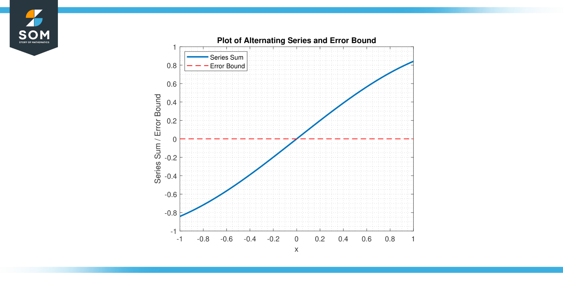
Figure-1.
This powerful tool is crucial in various mathematical fields, including numerical analysis, calculus, and applied mathematics, where approximations are commonly employed to tackle complex problems.
Process of Alternating Series Error Bound
Step 1: Consider a Convergent Alternating Series
To apply the alternating series error bound, we start with a convergent alternating series of the form:
S = a₁ – a₂ + a₃ – a₄ + a₅ – a₆ + …
where a₁, a₂, a₃, … are the terms of the series.
Step 2: Verify the Conditions for Convergence
Before proceeding, we must ensure that the alternating series satisfies the conditions for convergence. Two essential conditions are:
- The terms of the series must decrease in magnitude monotonically, meaning that |a₁| ≥ |a₂| ≥ |a₃| ≥ …
- The terms must approach zero as the index increases, i.e., lim(n→∞) aₙ = 0.
These conditions are crucial for the convergence of the series.
Step 3: Determine the Error in the Partial Sum
Let’s assume we want to approximate the value of the series S by considering the first n terms. The partial sum Sn is given by:
Sn = a₁ – a₂ + a₃ – a₄ + … + $-1^{n+1}$ * aₙ
The error in the partial sum, denoted as Rn, is the difference between the exact value of the series and its partial sum:
Rn = S – Sn
Step 4: Identify the Alternating Series Error Bound
The alternating series error bound states that the error in the partial sum is bounded by the magnitude of the first neglected term, i.e., the (n+1)th term:
|Rn| ≤ |aₙ₊₁|
This bound provides an upper limit on the error incurred when approximating the series.
Step 5: Determine the Maximum Error
To estimate the maximum error in the approximation, we seek the largest possible value for |aₙ₊₁| in the series. This typically occurs when |aₙ₊₁| is the largest among the terms. We can establish an upper bound on the error by identifying the term with the maximum magnitude.
Applications
Numerical Analysis
In numerical analysis, the alternating series error bound is utilized to evaluate the accuracy of numerical methods and algorithms. Approximations obtained through numerical methods frequently rely on series expansions, and the error bound enables analysts to quantify the precision of these approximations. By managing the error through the bond, mathematicians and scientists can ensure reliable and accurate numerical computations.
Calculus
The alternating series error bound holds a prominent position in calculus, especially in the context of Taylor series expansions. Taylor series approximates functions by expressing them as infinite series of terms. The error bound plays a vital role in assessing the accuracy of the approximation and assists in determining the number of terms required to attain a desired level of precision. Using the error bound, mathematicians can approximate functions and enhance the accuracy of evaluating integrals, derivatives, and differentials.
Applied Mathematics
In applied mathematics, the alternating series error bound is crucial in numerous modeling and simulation techniques. Many real-world phenomena are mathematically represented through series expansions, and the error bound quantifies these models’ accuracy. By considering the error bound, researchers can make informed decisions regarding the fidelity of their simulations and make appropriate adjustments to the parameters.
Signal Processing and Fourier Analysis
The Fourier series, a fundamental tool in signal processing and harmonic analysis, expresses periodic functions as infinite sums of trigonometric functions. The alternating series error bound estimates the truncation error when approximating a function using a finite number of Fourier series terms. This estimation is particularly useful in applications like audio and image compression, where a precise representation of signals is of utmost importance.
Probability and Statistics
In probability theory and statistics, the alternating series error bound is relevant when approximating probabilities and estimating statistical parameters. By utilizing series expansions, analysts can approximate intricate probability distributions and obtain valuable approximations for statistical calculations. The error bound measures the error in these approximations and aids in determining the necessary number of terms for achieving precise outcomes.
Exercise
Example 1
Consider the alternating series: S = 1 – 1/2 + 1/4 – 1/8 + 1/16 – 1/32 + … Find an approximation for the value of S that guarantees an error less than 0.01.
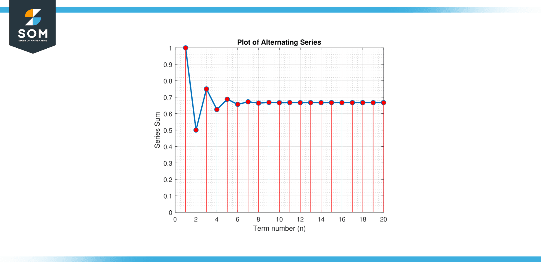
Figure-2.
Solution
We must determine the number of terms required to find an approximation with an error less than 0.01. Let’s apply the alternating series error bound. The terms of the series decrease in magnitude, and the limit of the terms as n approaches infinity is 0, satisfying the conditions for convergence. We can use the error bound:
|Rn| ≤ |aₙ₊₁|
Rn is the error, and aₙ₊₁ is the (n+1)th series term. In this case, |aₙ₊₁| = 1/2ⁿ⁺¹.
We want to find n such that |aₙ₊₁| ≤ 0.01. Solving the inequality gives 1/2ⁿ⁺¹ ≤ 0.01. Taking the logarithm base 2 of both sides, we get:
(n+1)log₂(1/2) ≥ log₂(0.01)
(n+1)(-1) ≥ -6.643856
n+1 ≤ 6.643856
n ≤ 5.643856
Since n must be a positive integer, we take the greatest integer less than or equal to 5.643856, which is 5. Therefore, we need to sum at least 6 terms to guarantee an error of less than 0.01.
Example 2
Find the minimum number of terms needed to approximate π to within an error of 0.001 using the alternating series expansion for π/4: π/4 = 1 – 1/3 + 1/5 – 1/7 + 1/9 – …
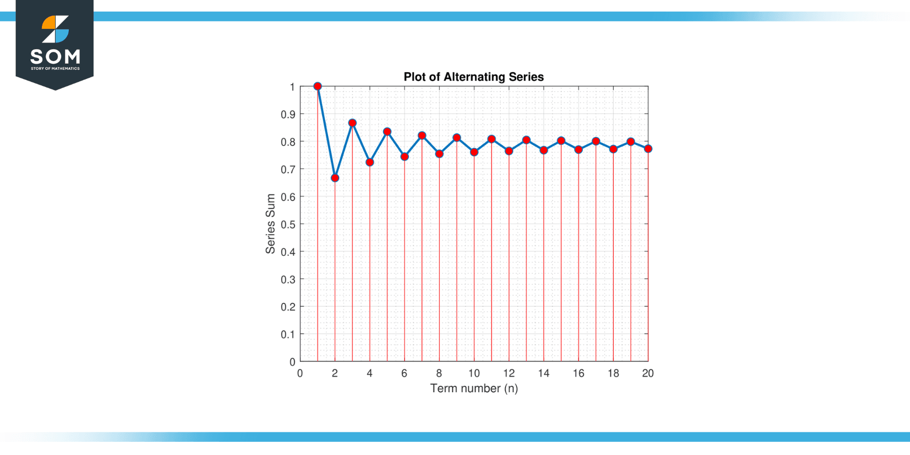
Figure-3.
Solution
We want to find the minimum number of terms to guarantee an error of less than 0.001. The error bound for this alternating series is |Rn| ≤ |aₙ₊₁|, where aₙ₊₁ is the (n+1)th term. In this case:
|aₙ₊₁| = 1/(2n+1)
We need to find n such that |aₙ₊₁| ≤ 0.001. Solving the inequality gives:
1/(2n+1) ≤ 0.001
2n+1 ≥ 1000
2n ≥ 999
n ≥ 499.5
Since n must be a positive integer, we take the smallest integer greater than or equal to 499.5, which is 500. Therefore, we need to sum at least 500 terms to approximate π to within an error of 0.001.
All images were created with GeoGebra and MATLAB.