JUMP TO TOPIC

In the intricate tapestry of calculus, the Mean Value Theorem for Integrals elegantly sews together fundamental concepts of integration and continuity. This theorem, an instrumental cornerstone of integral calculus, furnishes a powerful tool for deciphering the intricate interplay between areas under curves and average values of continuous functions.
With applications spanning from physics to economics, the Mean Value Theorem transcends the mathematical realm, providing tangible insights into the behavior of dynamic systems.
This article will delve into the theorem’s elegant proof, illustrious history, extensive applications, and far-reaching implications, illuminating its integral role in the broader context of mathematical understanding.
Definition of Mean Value Theorem for Integrals
In the realm of integral calculus, the Mean Value Theorem for Integrals stands as a vital principle, formally stating that if a function is continuous on the interval [a, b], then there exists at least one number c in this interval such that the integral of the function over the interval [a, b] is equal to the length of the interval multiplied by the function’s value at c. Mathematically, this can be expressed as:
$\int_{a}^{b} f(x) \, dx = (b – a) \cdot f(c)$
for some c in the interval [a, b].
In essence, the theorem states that there is at least one point within the specified interval where the function’s value equals the function’s average value over that interval. It elegantly bridges the gap between the local behavior of a function (i.e., its value at a specific point) and its global behavior (i.e., its integral over an interval).
Proof of Mean Value Theorem for Integrals
Let f(x) be a function continuous on a closed interval [a, b]. By definition, the average value of f(x) over the interval [a, b] is given by
A = $\frac{1}{b-a} \int_{a}^{b}$ f(x), dx
The function f(x), being continuous on [a, b], has an antiderivative F(x). Now, consider a new function G(x) = F(x) – A(x – a).
We can observe that G(a) = G(b):
G(a)=F(a)−A(a−a)=F(a),
G(b) = F(b) – A(b – a) = F(b) – $\int_{a}^{b}$ f(x), dx = F(a) = G(a)
By Rolle’s Theorem, since G(x) is continuous on [a, b], differentiable on (a, b), and G(a) = G(b), there exists some c in (a, b) such that the derivative of G at c is zero, i.e., G'(c) = 0.
Now, G'(x) = F'(x) – A = f(x) – A (since F'(x) = f(x) and the derivative of A(x – a) is A), which gives us
or equivalently
f(c) = A = $\frac{1}{b-a} \int_{a}^{b}$ f(x) , dx
This result states that there exists some c in [a, b] such that the value of f at c is the average value of f on [a, b], precisely the statement of the Mean Value Theorem for Integrals (MVTI).
Properties
The Mean Value Theorem for Integrals carries a host of properties and consequences that reveal fundamental aspects of calculus. Here, we delve into some of these attributes in greater detail:
– Existence of Average Value
The theorem guarantees that, for a function continuous on an interval [a, b], there exists at least one value c in that interval such that f(c) equals the average value of f on [a, b]. This shows that a continuous function on a closed interval always attains its average value at least once within the interval.
– Dependency on Continuity
The theorem’s requirement for f(x) to be continuous over the interval [a, b] is essential. Without continuity, the theorem might not hold. For example, consider a function that is always zero except at one point where it takes a large value. The average value over any interval is close to zero, but the function only reaches a high value at one point.
– Existence of a Tangent Parallel to the Secant
A geometric interpretation of the theorem is that for any continuous function defined on the interval [a, b], there’s a tangent to the function’s graph within the interval that is parallel to the secant line connecting the endpoints of the graph over [a, b]. In other words, there’s at least one instantaneous rate of change (the slope of the tangent) that equals the average rate of change (the slope of the secant).
Non-uniqueness of c
The Mean Value Theorem for Integrals ensures the existence of at least one c in the interval [a, b] for which the theorem holds, but there can be multiple such points. In fact, for some functions, there might be an infinite number of points satisfying the theorem’s conditions.
– Applications
The Mean Value Theorem for Integrals underpins many mathematical and real-world applications, such as proving inequalities, estimating the errors in numerical integration, and solving differential equations. In fields like physics and engineering, it’s instrumental in understanding phenomena described by continuous functions over an interval.
– Connection with Fundamental Theorem of Calculus
The Mean Value Theorem for Integrals is closely related to the First Fundamental Theorem of Calculus, as both explore the relationship between a function and its integral. In fact, the Mean Value Theorem for Integrals can be proven using the Fundamental Theorem.
By exploring these properties, we can glean the full impact of the Mean Value Theorem for Integrals and its pivotal role in deepening our understanding of calculus.
Limitations of Mean Value Theorem for Integrals
The Mean Value Theorem for Integrals is a powerful mathematical tool with broad applicability, yet it does have its limitations and requirements:
– Requirement for Continuity
The function under consideration must be continuous on the interval [a, b]. This is a key prerequisite for the theorem. Functions with discontinuities in the interval may not satisfy the theorem, limiting its application to functions that are discontinuous or undefined at points within the interval.
– Non-Specificity of c
The theorem guarantees the existence of at least one point c in the interval [a, b] where the integral of the function over the interval equals the length of the interval times the function’s value at c.
However, it does not provide a method for finding such a c, and there may be more than one such value. For some applications, not knowing the exact value can be a limitation.
– Limitation to Real-Valued Functions
The Mean Value Theorem for Integrals applies only to real-valued functions. It doesn’t extend to complex-valued functions or functions whose values lie in more general sets.
– No Guarantee for Maximum or Minimum
Unlike the Mean Value Theorem for Derivatives, the Mean Value Theorem for Integrals does not provide any information about where a function may achieve its maximum or minimum values.
– Dependence on Interval
The theorem holds for a closed interval [a, b]. If the function is not well-defined on such an interval, the theorem might not be applicable.
In general, while the Mean Value Theorem for Integrals is a valuable tool within the framework of calculus, it is essential to bear in mind these limitations when applying it. Understanding these boundaries helps ensure its correct and effective usage within mathematical and real-world problem-solving.
Applications
The Mean Value Theorem for Integrals (MVTI) is a cornerstone concept in calculus with wide-ranging applications across numerous fields. Its utility arises from its ability to bridge the gap between local and global behaviors of a function, enabling insightful analysis of various systems. Here are several applications across various fields:
– Mathematics
— Proofs and Theorems
MVTI is used in proving various theorems in calculus and analysis. For instance, it plays a crucial role in proving the First and Second Fundamental Theorems of Calculus, which are essential to integral calculus.
— Error Bounds
In numerical methods for approximating integrals, such as Simpson’s Rule or the Trapezoidal Rule, MVTI helps in estimating the error bounds. The theorem allows us to understand how far our approximations can be off, which is particularly important for ensuring the precision of calculations.
– Physics
— Motion and Kinematics
In physics, MVTI has numerous applications, especially in kinematics, where it can be used to link average velocity with instantaneous velocity. If a car travels a certain distance over a certain time, there must be some instant at which its speed is equal to its average speed.
– Economics
In economics, MVTI is often used in cost analysis. For instance, it can be used to show that there exists a level of output where the average cost of producing an item is equal to the marginal cost.
– Engineering
— Control Systems
In control systems engineering, MVTI helps to provide insights into the stability and behavior of system dynamics, particularly for systems modeled by ordinary differential equations.
– Computer Science
— Computer Graphics
In computer graphics and image processing, some algorithms use the principles behind MVTI to perform operations like blurring (which involves averaging pixel values) and other transformations.
In each of these areas, the Mean Value Theorem for Integrals provides a vital link between the integral of a function and the behavior of that function within a specific interval. This proves useful in a broad range of practical applications, extending the theorem’s reach beyond the realms of pure mathematics.
Exercise
Example 1
Let’s find a value c for the function f(x) = x² on the interval [0, 2].
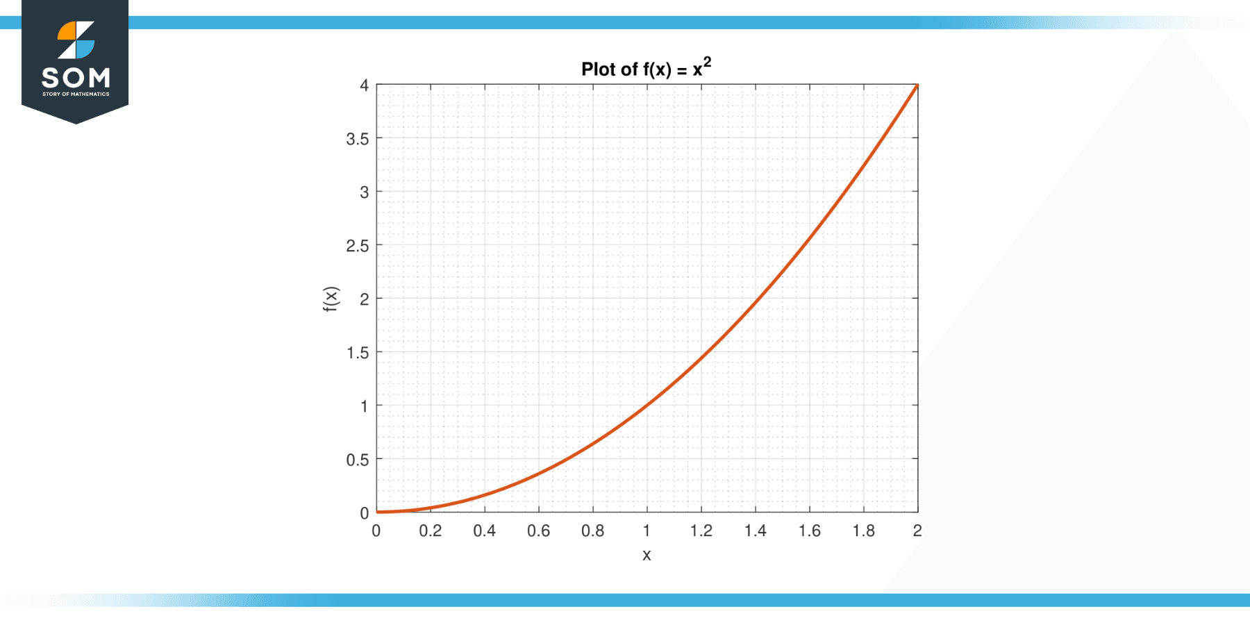
Figure-1.
Solution
The average value of f on [0, 2] is given by:
A = (1/(2-0)) $\int_{0}^{2}$ x² dx
A = (1/2) * $[x³/3]_{0}^{2}$
A = 8/3
By the MVTI, there exists a c in (0, 2) such that f(c) = A. We solve for c:
c² = 8/3
Yielding, c = √(8/3). Approximately 1.633.
Example 2
Consider the function f(x) = 3x² – 2x + 1 on the interval [1, 3].

Figure-2.
Solution
The average value of f on [1, 3] is given by:
A = (1/(3-1)) $\int_{1}^{3}$ (3x² – 2x + 1) dx
A = (1/2) * $[x³ – x² + x]_{0}^{2}$
A = 8
By the MVTI, there exists a c in (1, 3) such that f(c) = A. We solve for c:
3c² – 2c + 1 = 8
Yielding, c = 1, 2.
Example 3
Consider the function f(x) = sin(x) on the interval [0, π].
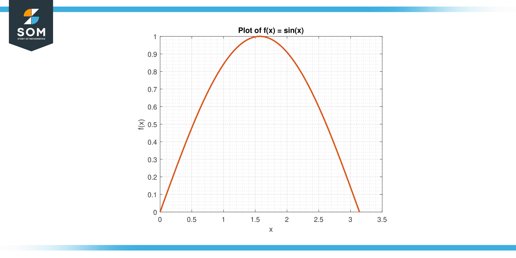
Figure-3.
Solution
The average value of f on [0, π] is given by:
A = (1/π) $\int_{0}^{π}$ sin(x) dx
A = (1/π) * $[-cos(x)]_{0}^{π}$
A = 2/π
By the MVTI, there exists a c in (0, π) such that f(c) = A. We solve for c:
sin(c) = 2/π
Yielding:
c = arcsin(2/π)
Approximately 0.636.
Example 4
Consider the function f(x) = eˣ on the interval [-1, 1].
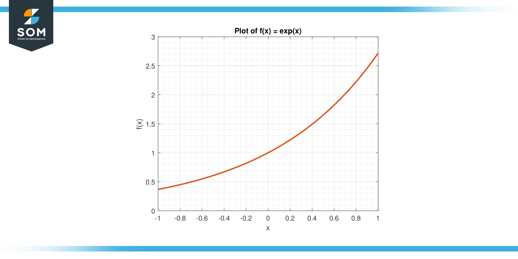
Figure-4.
Solution
The average value of f on [-1, 1] is given by:
A = (1/(1-(-1))) $\int_{-1}^{1}$ eˣ dx
A = (1/2) * $[e^x]_{-1}^{1}$
A = (e – e⁻¹)/2
Approximately 1.175.
By the MVTI, there exists a c in (-1, 1) such that f(c) = A. We solve for c:
eᶜ = (e – e⁻¹)/2
Yielding:
c = ln[(e – e⁻¹)/2]
Approximately 0.161.
Example 5
Consider the function f(x) = x³ on the interval [-1, 1].
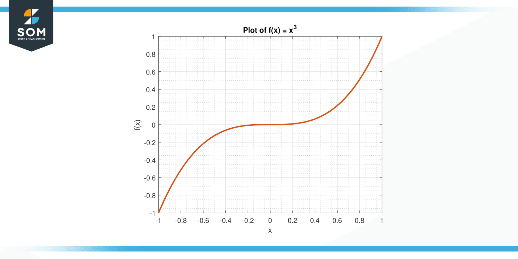
Figure-5.
Solution
The average value of f on [-1, 1] is given by:
A = (1/(1-(-1))) $\int_{-1}^{1}$ x³ dx
A = (1/2) * $[x⁴/4]_{-1}^{1}$
A = 0
By the MVTI, there exists a c in (-1, 1) such that f(c) = A. We solve for c:
c³ = 0
Yielding, c = 0.
Example 6
Consider the function f(x) = 1/x on the interval [1, e].
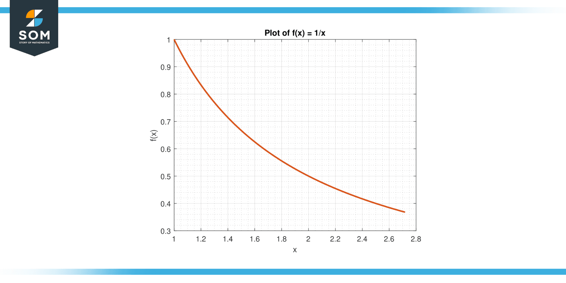
Figure-6.
Solution
The average value of f on [1, e] is given by:
A = (1/(e-1)) $\int_{1}^{e}$ 1/x dx
A = (1/(e-1)) * $[ln|x|]_{1}^{e}$
A = 1
By the MVTI, there exists a c in (1, e) such that f(c) = A. We solve for c:
1/c = 1
Yielding c = 1.
All images were created with MATLAB.