JUMP TO TOPIC
- What Is Applied Calculus?
- Applied Calculus vs Calculus
- Who Should Study Applied Calculus?
- Applied Calculus Topics
- Function
- Linear Function
- Non-Linear Functions
- Domain of a Function
- Range of a Function
- Open Interval of a Function
- Closed Interval of a Function
- Example 1:
- Solution:
- Example 2:
- Solution:
- Example 3:
- Solution:
- Example 4:
- Solution:
- Example 5:
- Solution:
- Inverse Function
- Example 6:
- Solution:
- Example 7:
- Solution:
- Derivative
- Limits and Continuity
- Example 8:
- Solution:
- Example 8:
- Solution:
- Example 9:
- Solution:
- Differentiation of a Function
- Example 10:
- Solution:
- Differential Rules of Function
- Example 11:
- Solution:
- Example 12:
- Solution:
- Example 13:
- Solution:
- Example 15:
- Solution:
- Example 16:
- Solution:
- Example 17:
- Solution:
- Integral Calculus
- Example 18:
- Solution:
- Example 19:
- Solution:
- Example 20:
- Solution:
- Example 21:
- Solution:
- Practice Questions:
- Answer Keys
 “Applied Calculus” is a single-level course that covers the basics of several topics such as functions, derivatives and integrals.
It is also known as “baby calculus” and discusses several topics which are also part of a calculus course. In this topic, we will discuss applied calculus, its similarities and differences with calculus, and its related examples.
This topic should not be taken as an applied calculus book as we will only discuss specifics topics along with some applied calculus examples. Furthermore, we will study the basics of functions, derivatives and integrals as part of applied calculus.
What Is Applied Calculus?
Applied Calculus, also known as “baby calculus or business calculus,” is an introductory level course that covers the basics of several topics such as functions, derivatives and integrals.
It does not include trigonometry or advanced algebra, which are studied in Calculus I and II. High school algebra can be considered a prerequisite for Applied Calculus.
Applied Calculus vs Calculus
The main difference between Applied Calculus and Calculus is that Applied Calculus covers the basics of functions, derivatives and integrals but skips advanced topics related to derivatives and integration, which falls under Calculus. Calculus applied is simple, and it does not include the the high-level calculus that scientists and engineers study.
Students who choose to study calculus are mostly engineering or science students, and they study calculus in two parts; calculus – I and calculus –II. Both these courses are covered in two semesters or a year. On the other hand, applied calculus is studied mainly by economics and business administration students as their field does not involve complex calculus.
The general course contents of applied calculus, pre-calculus, calculus – I, and calculus –II are presented below.
Applied Calculus
It does not include any topics from trigonometry. It has the least amount of theorems compared to the rest of the calculus subjects, and it does not include a discussion of complex algebraic functions.
Major topics of applied calculus include:
- Functions
- Derivatives
- Applications of derivatives
- Simple Integration
- Simple multivariable calculus
Pre-Calculus
As the name suggests, pre-calculus is the pre-requisite for applied calculus, calculus –I, and calculus –II. Pre-calculus only deals with functions, and the topics related to pre-calculus are revised before starting the applied calculus course. So both pre-calculus and applied calculus include a discussion of procedures.
The major topics of pre-calculus are:
- Linear Functions
- Inverse Functions
- Operations on Functions
- Complex numbers and roots
- Polynomial functions
Calculus – I
Calculus’ main focus is on limits, continuous functions, differentiation, and applications related to differentiations such as mean value theorems, Rolle’s theorem, extreme value theorem, etc.
Major topics of calculus-I are:
- Derivatives
- Limits and derivative applications
- Partial differentiation
- Integration
- Applications of integration
Calculus – II
Calculus-II is an advanced form of calculus-I, and it includes topics that are specifically included in the curriculum of engineering and science students. Calculus-II is used to study change or continuous motions presented in the form of functions.
Major topics of calculus-II include:
- Differential equations and their applications
- Complex functions
- Binomial series
- Sequences, series and geometric functions
- Analytical geometry
The subject-wise fundamental differences in the course outlines included in applied calculus and calculus are presented in the table below. The table can be used as a side-by-side course outline comparison between applied calculus and calculus.
| Topics | Applied Calculus | Calculus |
| Advance or analytical Geometry | Not included | Included |
| Trigonometry | Not Included | Included |
| Functions | Linear, Quadratic and polynomial functions are included. Basic level logarithmic and exponential functions are sometimes included as well. | Polynomial, linear, logarithmic, exponential, and integral functions are included. |
| Derivatives | Simple algebraic derivatives, chain rule, and applied optimization | Included |
| Advance Differential equations | Not included | Included |
| Integration | Basic Integration, Anti-derivatives, and calculation of area and volume using integration | Algebraic Integration, Advance integration via substitution method |
| Limits and continuous functions | Basic graphical and numerical | Advance graphical, numerical, and algebraic functions. |
History of Calculus
Modern-day calculus was developed by none other than Sir Isaac Newton and Gottfried Leibniz. These scientists studied the continuous motions of planets and moons, so the name “calculus of the infinitesimal” was coined. Calculus of the infinitesimal means studying continuous changes using mathematics.
Since the development of calculus in the 17th century, many other scientists have contributed to calculus, and it has evolved. Many new methods, theorems, and hypotheses have been presented, and now calculus is applied in physics, biology, economics and engineering.
The beauty of calculus is that it is easy to understand and presents some basic and simple ideas which we can apply to many everyday scenarios. When we use calculus for simple real-life problems, it becomes applied calculus.
Who Should Study Applied Calculus?
We have discussed the similarities and differences between applied calculus and calculus, so now a question arises: who should study applied calculus? Applied calculus has its applications, and even if it is called “baby calculus,” there is no denying the significance of studying this course.
The list of schools/colleges where applied calculus is preferred over calculus is given below:
- Pre-medical schools
- Pharmacy schools
- Business and administration schools
- Non-research graduate-level programs
- Applications of Applied Calculus
The next question that comes to the mind of students is, “Is applied calculus hard?” The answer to this question is that it is simpler and easier as compared to calculus -I and II. The applications of applied calculus vary significantly from that of calculus. Engineers and scientists use calculus to solve advanced geometrical problems, find volumes and distances of complex functions, derive theorems, and solve advanced multivariable calculus problems.
On the contrary, applied calculus is mainly used by economic and business personnel to determine the maximum or minimum profits, find or calculate the elasticity of demand, and calculate income stream flows and break-even points in cash flows using basic calculus.
Applied Calculus Topics
Function
Function, in calculus, is defined as the relation between two variables where one variable will be dependent and the other one will be independent. The value of the dependent variable will vary according to the value of the independent variable. For example, the function equation is represented like this if “x” is the independent variable and “y” is the dependent variable:
$ y = f(x)$
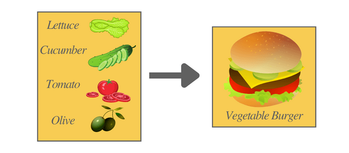
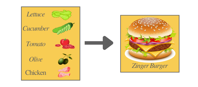
In generic terms, we can say that the function’s output will be dependent on the input. For example, we want to make a burger. If we only add lettuce, tomatoes, cucumbers, and olives, we will get a vegetable burger, but if we’re going to make a zinger burger, we will have to add chicken. So as you can see, the input ingredients define the type of burger.
Hence, the kind of burger is a dependent variable, while the ingredients are the independent variables. The mapping from the inputs to the outputs is called a function.
Linear Function
A linear function is extensively used in the field of economics. It is popular in economics as it is easy to use and graphs are easy to understand. The variables in the linear functions will be without the exponents; this means that all the variables will have the power of “1.”
The listed equations below are examples of a linear function:
- $y = 3x$
- $y = 3x +2$
- $y = 6x -2$
Non-Linear Functions
A non-linear function is also a relationship between dependent and independent variables, but unlike a linear function, it will not form a straight line. Quadratic functions, cubic functions, exponential functions, and logarithmic functions are examples of non-linear functions. Equations listed below are examples of a non-linear function.
- $y = 3x^{2}$
- $y = e^{2x}$
- $y = \dfrac{1}{x^{3}}$
- $y = ln(3x)$
Domain of a Function
The domain of a function is defined as the set of all possible inputs of the function. It can also be defined as all possible values of the independent variable.
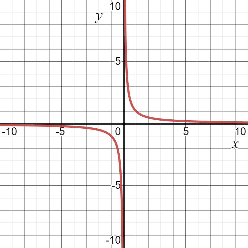
Let us look at an example — for the function $y = \dfrac{1}{x}$, the value of “$y$” will be infinity or undefined at $x = 0$. Other than that, it will have some value. Because of this, the domain of the function will be all the values of “$x$,” i.e., all real numbers except $x = 0$.
Range of a Function
The range of a function is defined as the set of all possible outputs of a function. It can also be defined as all possible values of the dependent variable. If we take the same numerical example $y = \dfrac{1}{x}$, then the range of the function will also be any value other than zero. The graph below shows the values of both “$x$” and “$y$,” and it can be seen by the curve that “$y$” can have any value except “$0$”.
Open Interval of a Function
The open interval can be defined as an interval that includes all the points within the given limit except both the endpoints, and it is denoted by ( ). For example, if the function $y = 3x +2$ is defined for the interval $(2, 4)$, then the value of “$x$” will include all the points greater than $2$ and less than $4$.
Closed Interval of a Function
The closed interval can be defined as an interval that includes all the points within the given limit, and it is denoted by [ ]. For example, if the function y = 3x +2 is defined for the interval $[2, 4]$, then the value of “x” will include all the values greater than or equal to $2$ and less than or equal to $4$.
Example 1:
From the data given below, determine the value of $f(3)$ for the function $y = f(x)$
| X | $1$ | $2$ | $3$ | $4$ | $5$ |
| Y | $2$ | $4$ | $6$ | $8$ | $10$ |
Solution:
We can clearly see from the table that $f(3) = 6$.
Example 2:
Express the equation $6x – 3y = 12$ as a function $y = f(x)$.
Solution:
$ 6x – 3y = 12$
$ 3 (2x-y) = 12$
$ 2x – y = \dfrac{12}{3}$
$ 2x – y = 4 $
$ y = f(x) = 2x – 4$
Example 3:
Solve the function $f(x) = 6x +12$, at $x = 3$
Solution:
$f(x) = 6x +12$
$f(3) = 6 (3) +12$
$f(3) = 18 + 12 = 30$
Example 4:
Solve the function $f(x) = 6x^{2} +14$, at $x = 2$
Solution:
$f(x) = 6x^{2} + 14$
$f(2) = 6 (2)^{2} + 14$
$f(2) = 6 (4) + 14$
$f(2) = 24 + 14 = 38$
Example 5:
Find out the domain and range of the following functions.
- $f(x) = 2x + 4$
- $f(x) = \sqrt{x+4}$
- $f(x) = \dfrac{6}{4x – 8}$
Solution:
1) For the function $f(x) = 2x + 4$, there are no restrictions. The variable “$x$” can take any value, and the result will always be a real number, hence the domain of the function will be $(-\infty, \infty)$.
The range of the function will also have no restrictions as for any value of “$x$” the function can take any real value, so the range of the function is also $(-\infty, \infty)$.
2) It is an irrational function, and we cannot take or solve the square root of a negative number. Hence, the value of “x” must be greater or equal to $-4$, so the function’s domain is given as $[-4, \infty)$. We started the domain with a closed interval bracket and ended it with an open interval, so “$x$” can take any value greater than $-4$ and less than infinity.
We have to look at the function’s minimum and maximum possible output to determine the range. The function can achieve values from “$0$” to infinity for the given domain. Hence, the range of the function is $[0, \infty)$.
3) The function will be real values except at $x = 2$, which will be indefinite. Hence, the domain of the function will be $( – \infty , 2) U (2, \infty)$. For this domain, the function’s output will never be zero, so the range of the function will be $(-\infty, 0) U (0, \infty)$.
Inverse Function
The inverse of a function is basically the reciprocal of the original function. If the original function is $y = f(x)$, then its inverse will be given as $x = f(y)$. The inverse function is denoted as $f^{-1}$.
We have studied most of the basics related to the topic of functions along with numerical examples. Let us now take a look at a real-life example related to functions.
Example 6:
Steve has a library in his house containing $400$ books. He purchases $10$ books monthly and adds them to his collection. You must write the formula for the total number of books (in the form of function $y = f(x)$). Is the function for the number of books linear or nonlinear? You must also determine the total amount of books at the end of $2$ years.
Solution:
In this example, we have a constant value of $400$ books already present in the library. Steve adds $10$ books monthly, so these $10$ books are the rate of change, and “$x$” will be the number of months.
We can then write the equation as:
$y = 400 + 10 (x)$
We can see from the above equation that it is a linear function. We have to determine the total number of books at the end of $2$ years.
$x = 2$ years $= 24$ months.
$y = 400 + 10 (24) = 400 + 240 = 640$ books
Example 7:
Let us modify the above example. Suppose Steve is pretty selective in buying books, and he has the money to buy $0$ to $10$ books monthly. His library already contains $400$ books. Write the number of books “$y$” at the end of the year in the form of an equation and determine the domain and range of the function.
Solution:
We can write the function as:
$y = 400 +12 x$
Here, $12$ is the number of months in a year.
The value of “$x$” can vary from $0$ to $10$, so the function’s domain will be $[0,10]$. The range of the function will be $[400, 520]$.
Derivative
In mathematics, more importantly in differential calculus, the derivative is defined as the rate of change of a function for a given variable. The derivative of a function $f(x)$ is denoted by $f'(x)$.
We can easily explain the idea of a derivative through the example of a slope. If we draw a straight line in the $x-y$ plane, then the change in the value of “$y$” for changes in the value of “x” gives us the slope.
Slope from point A to B is given as m $= \dfrac{y_2\hspace{1mm}-\hspace{1mm}y_1}{x_2\hspace{1mm}-\hspace{1mm}x_1}$
So if we keep the definition of slope in mind, then we can define derivative as:
1. The derivative is the slope of the tangent line of the function $y = f(x)$ at a given point $(x, y)$ or $(x,f(x))$.
2. The derivative can also be defined as the slope of the curve of the function $y = f(x)$ at the point $(x,y)$ or $(x, f(x))$.
Limits and Continuity
The limit of a function is used when the variable used in the function does not have a specific value; instead, it is close to a certain value. Suppose function $f(x)$ is defined for an open interval close to the number “$c$”. So when “x” approaches “$c$,” the value of the function is, let’s say, “$L$.” Then, the symbolic representation of this function is given as:
$\lim_{x \to \ c} f(x) = L$
The above equation tells us that $f(x)$ gets closer and closer to value $L$ when “$x$” approaches “$c$”.
Right-hand Limit:
For the right hand limit, we will write $\lim_{x \to \ c^{+}} f(x) = M$. This means that the value of the function $f(x)$ will be approaching “$M$” when “x” approaches “$c$” from the right side, i.e., the value of “$x$” will always be very close to “$c$” but it will always be greater than “$c$.”
Left-hand Limit:
The left-hand limit exists when the value of the function is determined by approaching the variable from the left side. It is written as $\lim_{x \to \ c^{-}} f(x) = L$, so the value of $f(x)$ is close to $L$ when “$x$” approaches “$c$” from the left side, i.e., “$x$” is close to but smaller than “$c$.”
Continuity of a Function:
A function is said to be continuous at $x = c$ if it satisfies the following three conditions:
1. The value $f (c)$ is defined.
2. $\lim_{x \to \ c} f(x)$ should exist, i.e., $\lim_{x \to \ c^{-}}f(x) = \lim_{x \to \ c^{+}}f(x)$
3. $\lim_{x \to \ c} f(x) = f (c)$
Example 8:
Determine whether $\lim_{x \to \ 3} f(x)$ exists for a given function:
$f(x) = \begin{cases}
& 3x+2 \quad 0<x<3 \\
& 14-x \quad 3<x<6
\end{cases}$
Solution:
The left hand limit of the function will be written as:
$\lim_{x \to \ 3^{-}} f(x) = \lim_{x \to \ 3^{-}} (3x+2)$
$\lim_{x \to \ 3^{-}} (3x+2) = {3(3) + 2} = 11$
$\lim_{x \to \ 3^{+}} f(x) = \lim_{x \to \ 3^{-}} (14-x)$
$\lim_{x \to \ 3^{-}} (14-x) = 14 – 3 = 11$
So, since $\lim_{x \to \ 3^{-}}f(x) = \lim_{x \to \ 3^{+}} f(x)$
The $\lim_{x \to \ 3} f(x)$ exists and it is equal to $11$
Example 8:
Discuss whether or not function $f(x) = 4x^{2} + 6x -7$ is continuous at $x = 2$.
Solution:
$\lim_{x \to \ 2} f(x) = \lim_{x \to \ 2} ( 4x^{2} + 6x -7)$
$\lim_{x \to \ 2} ( 4x^{2} + 6x -7) = 4(2)^{2}+ 6(2) -7) = 16 +12 -7 = 21$
$f(2) = ( 4x^{2} + 6x -7) = 4(2)^{2}+ 6(2) -7) = 21$
$\lim_{x \to \ 2} f(x) = f(2)$
Hence, the function is continuous at $x =2$.
Example 9:
Discuss whether or not the given function $f(x)$ is continuous at $x = 2$.
$f(x) = \begin{cases}
& 3x-4 \quad x<2 \\
& 10-x \quad 2 \leq x
\end{cases}$
Solution:
The left hand limit of the function will be written as:
$\lim_{x \to \ 2^{-}} f(x) = \lim_{x \to \ 2^{-}} (3x-4)$
$\lim_{x \to \ 2^{-}} (3x-4) = {3(2) – 4} = 2$
$\lim_{x \to \ 2^{+}} f(x) = \lim_{x \to \ 2^{+}} (10-x)$
$\lim_{x \to \ 2^{+}} (10-x) = 10 – 2 = 8$
Since $\lim_{x \to \ 2^{-}}f(x) \neq \lim_{x \to \ 2^{+}} f(x)$, II condition is not satisfied and hence the function f(x) is not continuous at $x =2$.
Differentiation of a Function
In calculus, the differentiation of a real-valued continuous function is defined as the change in function with respect to change in the independent variable. If you noticed, we have used the word continuous in the definition as differentiation of function can only be possible if it is continuous. The derivative of a function is denoted as $f'(x)$ and its formula is given as:
$\dfrac{d}{dx}f(x) = \dfrac{df}{dx}= \dfrac{dy}{dx}$
The algebraic representation of differentiation of a function in terms of limit can be given as:
$f'(x) = \lim_{c \to \ 0} \dfrac{f(x+c)-f(x)}{c}$
Proof:
Consider a continuous (real – valued) function “$f$” in an interval $(x, x_1)$. The average rate of change for this function for the given points can be written as:
Rate of change $= \dfrac{f(x_1)-f(x)}{x_1 – x}$
If the variable “$x_1$” is in the neighborhood of “$x$”, we can say that “$x_1$” is approaching “$x$”.
So we can write:
$\lim_{x \to \ x_1} \dfrac{f(x_1)-f(x)}{x_1 – x}$
We assumed that the function is continuous, so this limit will exist as it is one of the conditions for the continuity of a function. If the limit exists, we can write this function as $f'(x)$
If $x_1- x = c$, as “$x_1$” is in the neighborhood of “$x$”, the value of “$c$” should be approaching zero and we can write:
$\lim_{c \to \ 0} \dfrac{f(x+c)-f(x)}{c}$
So if this limit exists, then we say its instantaneous rate of change of “$x$” for “$x$” itself and is denoted by $f’ (x)$.
Steps of Finding the Derivative:
If a real-valued continuous function “$f$” is given, then $f’ (x)$ can be determined by following the given steps:
1. Find $f(x+h)$.
2. Solve for $f(x+h) – f(x)$.
3. Divide the equation in step 2 by “h”.
4. Solve for $\lim_{h \to \ 0} \dfrac{f(x+h)-f(x)}{h}$.
Example 10:
Find the derivative of the function $y = x^{3}- 3x + 6$ at $x = 3$ using the limit method.
Solution:
$= (x+h)^{3}-3(x+h) +6$
$= {(x+h)^{3}-3(x+h) +6} – (x^{3}- 3x + 6)$
$= [(x+h)^{3}- x^{3} ] – [3 {(x+h) – x} ] + [6 – 6]$
$= [(x+h) – x ] [(x+h)^{2}+ x^{2} + (x+h) x] -3h$
Dividing both sides by “h” and putting the limit such as h approaches to zero:
$f'(x) = \lim_{h \to \ 0} \dfrac{[(x+h) – x ] [(x+h)^{2}+ x^{2} + (x+h) x] -3h }{h}$
$f'(x) = \lim_{h \to \ 0}\dfrac{h [(x + h)^{2}+ (x + h) x + x^{2}] -3h }{h}$
$f'(x) = \lim_{h \to \ 0}\dfrac{h ([(x + h)^{2}+ (x + h) x + x^{2}] – 3) }{h}$
$f'(x) = \lim_{h \to \ 0}{ ([(x + h)^{2}+ (x + h) x + x^{2}] – 3) }$
$f'(x) = (x)^{2}+ (x). (x) + x^{2} – 3$
$f'(x) = 3x^{2} – 3$
$f'(3) = 3 (3) ^{2} – 3 = 27 – 3 = 24$
Differential Rules of Function
There are various types of functions, and we can find the derivative of each function by using different differential rules. By using the limit method, we can define the following rules for the differential of a function:
1. Differentiation of a constant function
2. Differentiation of a power function, also known as the power rule
3. Differentiation of a product function (Product Rule)
4. Differentiation of exponential function
5. Differentiation of summation and subtraction functions
6. Differentiation of a quotient function (Quotient Rule)
Let’s have a look at some examples.
Example 11:
Calculate the derivative of the constant function $f(c) = 6$.
Solution:
The derivative of a constant function is always zero
$f'(c) = \dfrac{dy}{dx} 6 = 0$
Example 12:
Calculate the derivative of the function $f(x) = 4x ^{\dfrac{3}{4}}$.
Solution:
$f(x) = 4x ^{\dfrac{3}{4}}$.
Taking derivative with respect to variable “$x$”
$f'(x) = 4 \times (\dfrac{3}{4}) x ^{(\dfrac{3}{4})-1}$ ( Power Rule)
$f'(x) = 3 x ^{\dfrac{3}{4}-1}$
$f'(x) = \dfrac{3}{x}$
Example 13:
Let us again take the same function of example 10 and verify the answer using different differentiation rules.
Solution:
$f(x) = x^{3}- 3x + 6$
We will use the combination of addition, subtraction and power rule of derivatives to solve this function.
Taking derivative on both sides with respect to “$x$”:
$f'(x) = 3x^{2} – 3 + 0$
We have to calculate the value of $f'(x)$ at $x = 3$.
$f'(3) = 3(3)^{2} – 3$
$f'(3) = 27 – 3 = 4$
The limits and continuity of the function are used to define derivatives, and then we have determined some rules to solve the problems related to the differentiation of functions quickly. Let us now look at some real-life examples of derivatives.
Example 15:
The function or formula for the height of an object is given as $d(t) = -8t^{2}+ 36 t +30$, where t is the time in seconds and d is the distance in meters. Suppose the object is thrown 30 meters above the ground level with a velocity of $50 \dfrac{m}{sec}$. What will be the maximum height of the object?
Solution:
Velocity is defined as the rate of change of position of an object for time. Hence, if any entity covers a distance from one point to another with respect to time, and if we take the derivative of that function, it will give us velocity.
So taking the derivative of $d(t) = -8t^{2}+ 36 t +30$ will give us velocity.
$v = d'(t) = -16t + 36$
The velocity of an object at the highest point is equal to zero.
$v = d'(t) = -16t + 36 = 0$
$-16t +36 = 0$
$t = \dfrac{9}{4} = 2.25$ sec
So the highest point or the distance covered above the ground by the object will be:
$d(2.25) = -8(2.25)^{2}+ 36 (2.25) +30 = -40.5 + 81 + 30 = 70. 5$ meters
Example 16:
Suppose a company $XYZ$ manufactures soap. The demand for their product can be given as the function $f(x) = 400 – 5x – 5 x^{2}$, where “$x$” is the price of the product. What will be the marginal revenue of the product if the price is set to $5$?
Solution:
The marginal revenue of the product will be calculated by taking the derivative of the revenue function.
Revenue of the product will be equal to the product of the price and quantity. If $f(r)$ is the function for the revenue, then it will be written as:
$f(r) = f(x) . x$
$f(r) = [400 – 5x – 5 x^{2}]. x$
$f(r) = 400x -5x^{2} – 5 x^{3}$
$f'(r) = 400 – 10x – 5 x^{2}$
$f'(r) = 400 – 10 (5) – 5 (5)^{2}$
$f'(r) = 400 – 50 – 125 = 225$
So this means that if the product’s price is set at $5$, then the revenue will increase by $225$.
Example 17:
Allan is a mathematics student, and he recently got a job in the national health care system. Allan is tasked to estimate the growth of the coronavirus in one of the country’s major cities. The growth rate function for the virus is $g(x) = 0.1e^{\dfrac{x}{2}}+ x^{2}$, where “$x$” is given in days. Allan needs to calculate the growth rate from the first week to the end of the second week.
Solution:
Allan needs to calculate the growth rate at the end of the first week and then at the end of the second week. After that, taking the ratio of both the growth rates, Allan will be able to tell how fast the virus is growing.
$g ( x) = 0.1e^{\dfrac{x}{2}}+ x^{2}$
$g'(x) = \dfrac{0.1}{2} e^{\dfrac{x}{2}} + 2x$
$g'(7) = 0.05 e^{\dfrac{7}{2}} + 2 (7) = 15.66$
$g'(14) = 0.05 e^{\dfrac{14}{2}} + 2 (14) = 82.83$
$\dfrac{ g'(14)}{ g'(7)} = 5$ approx.
So the growth rate of the coronavirus will be $5$ times higher at the end of $14$ days (second week) as compared to the end of $7$ days (first week).
Integral Calculus
Integral calculus is used to study integrals and properties associated with it. Integral calculus combines smaller parts of a function and then combines them as a whole.
How can we find the area under the curve? Can we determine the original function if a function’s derivative is given? How can we add infinitely small functions? The integral calculus provides the answers to all these questions, so we can say that integral calculus is used for finding the anti-derivative of $f’ (x)$.
We are finding the area under the curve for any function.
Integration
Integration is defined as the anti-derivative of a function. If derivative was used to segregate a complicated function into smaller parts, then integration is the inverse of derivative as it combines the smaller elements and makes them a whole. Its primary application is to find the area under the curve.
There are two types of integration:
1. Definite integrals
2. Indefinite integrals
Definite Integrals
The definite integral is the type of integration that follows a specific limit or certain boundaries during integration calculation. The upper and lower limits for the function’s independent variable are defined in the case of definite integrals.
$\int_{a}^{b}f(x).dx = F(b) – F(a)$
Indefinite Integrals
The indefinite integral is defined as the type of integration that does not use upper and lower boundaries. This integration results in a constant value added to the anti-derivative, and it is represented as follows:
$\int f(x).dx = F(x) + c$
Important integral formulas
This section will cover important integral formulas for both definite and indefinite integrals used in applied calculus. As applied calculus does not include trigonometry, we will not involve trigonometry formulas.
1. $\int x^{n}.dx = \dfrac{x^{n+1}}{n+1} + c$
2. $\int (ax+b)^{n}.dx = \dfrac{(ax+b)^{n+1}}{a(n+1)} + c$
3. $\int 1. dx = x + c$
4. $\int e^{x}. dx = e^{x} + c$
5. $\int b^{x}.dx = (\dfrac{b^{x}}{log b})$
6. $\int_{a}^{b}f'(x).dx = f(b) – f(a)$
7. $\int_{a}^{b}f(x).dx = – \int_{a}^{b}f(x).dx $
8. $\int_{-a}^{a}f(x).dx = 2 \int_{0}^{a}f(x).dx$, with the condition that function should be even
9. $\int_{-a}^{a}f(x).dx = 0$, with the condition that function should be odd
Example 18:
Evaluate the following integral functions:
- $\int (x^{2} – 3x + 6) dx$
- $\int (\dfrac{x}{x+4}) dx$ , $(x >4)$
- $\int (6x^{5} – 14\sqrt{x} + 18) dx$
Solution:
1.
$\int (x^{2} – 3x + 6) dx$ = $\int x^{2}.dx – \int 3x.dx + \int 6.dx$
$= \dfrac{x^{3}}{3} – 3 \dfrac{x^{2}}{2} + 6x + c $
2.
$\int (\dfrac{x}{x+4}) dx$ = $\int (\dfrac{x+ 4 – 4}{x+4}) dx$
= $\int 1 – \dfrac{4}{x+4} dx$
= $\int 1.dx – 4 \int (x+4)^{-1}.dx$
= $x – 4 ln (x+4) + c$
3.
$\int (6x^{5} – 14\sqrt{x} + 18) dx$
$= \int 6x^{5}.dx -\int 14 \sqrt{x}.dx + \int 18.dx$
$= \int 6x^{5}.dx -\int 14 x^{\dfrac{1}{2}}.dx + \int 18.dx$
$= 6 \dfrac{x^{6}}{6} – 14 x^{\dfrac{3}{2}} + 18x + c$
Example 19:
Evaluate the following integral functions:
- $\int_{1}^{4}(3+x). dx$
- $\int_{-1}^{4}x^{4} +3x^{2}. dx$
Solution:
1.
$\int_{1}^{4}(3+x). dx$
= $\int_{1}^{4}3.dx + \int_{1}^{4}x.dx$
= $[3x] _ {1}{4} + [ \dfrac{x^{2}}{2}] _ {1}{4}]$
= $[ 3(4) – 3(1) ] + [ \dfrac{4^{2}}{2} -\dfrac{1^{2}}{2} ]$
= $(12 – 3) + [(\dfrac{16}{2}) – \dfrac{1}{2}]$
= $9 + (8 – \dfrac {1}{2} )$
= $9 – \dfrac{15}{2} = \dfrac{3}{2}$
2.
$\int_{-1}^{4}x^{4} +3x^{2}. dx$
= $\int_{-1}^{4}x^{4}.dx + \int_{-1}^{4} 3x^{2}.dx$
= $[\dfrac{x^{5}}{5}] _ {-1}{4} + 3 [ \dfrac{x^{3}}{3}] _ {-1}{4}]$
= $[ \dfrac{4^{5}}{5}- \dfrac{(-1)^{5}}{5}] + 3 [ \dfrac{4^{3}}{3} -\dfrac{(-1)^{3}}{3} ]$
= $[\dfrac{1024}{5} + \dfrac{1}{5}] + 3 [ \dfrac{64}{3} + \dfrac{1}{3} ]$
= $205 +65 =270$
Example 20:
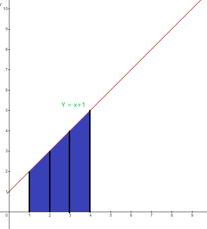
Determine the value of the highlighted area under the graph for the function $y = x +1$.
Solution:
The blue area under the graph has the lower limit of “$1$” and the upper limit of “$4$”. The integral function of the graph can be written as:
$\int_{1}^{4} ( x+1).dx$
Area $= \int_{1}^{4} x. dx + \int_{1}^{4} 1.dx$
= $[\dfrac{x^{2}}{2}] _{1}^{4} + [x] _ {1}^{4}$
= $[ \dfrac{16}{2}- \dfrac{1}{2}] + (4-1)$
= $(8- \dfrac{1}{2}) + 3$
= $\dfrac{15}{2} + 3$
= $\dfrac{21}{2}$ square units
Example 21:
Mason is studying the decaying rate of a bacterial infection in patients. The infection is decreasing at a rate of $-\dfrac{12}{(t + 3)^{2}}$ per day. On the 3rd day of their treatment, the infection percentage in patients was 3 (i.e., 300%). What will be the percentage of infection on the 15th day?
Solution:
Let “y” be the percentage of infection and variable “t” is for the number of days.
Rate of change of infection is given as $\dfrac{dy}{dt} = -\dfrac{6}{(t + 3)^{2}}$.
$\int dy = -12 \int (t+3)^{-2} dt$
$y = 12 (t+3)^{-1}+ c$
$y = \dfrac{12}{t+3} + c$
We know on the third day $ t = 3$ and $y = 3$
$3 = \dfrac{12}{3+3} + c$
$3 = 2 + c$
$c = 1 $
So now we can calculate the infection percentage on the 1st day.
$y = \dfrac{12}{15 + 3} + 1$
$y = \dfrac{12}{18} + 1$
$y = \dfrac{2}{3} + 1 = 0.6 + 1$ = $1.6$ or $160\%$
The infection rate reduced by $140 \%$ .
Practice Questions:
1. Suppose Simon throws a ball upwards at an initial velocity of $40 \dfrac{m}{s}$ while standing on the ground. Taking gravity into account, find the data given below:
- The time it would take for the ball to strike the ground
- The maximum height of the ball
2. The number of corona patients in city $XYZ$ for the year $2019$ was $3,000$; the number of patients is expected to double in $4$ years. Write the function y for the number of patients in $t$ years. After developing the function, you are also required to find:
- The total number of patients in $4$ years (after the formation of function)
- The time it would take to reach $60,000$ patients
Answer Keys
1.
- $8$ sec approx.
- $81.6$ meters
2.
The function can be written as $y = 3,000. 2^{\dfrac{t}{4}}$
- $6,000$ patients
- $17.14$ years approx.