JUMP TO TOPIC

Delving into the depths of linear algebra, one encounters the powerful Gram-Schmidt Process, a mathematical algorithm that transforms a set of vectors into an orthogonal or orthonormal basis.
It’s a fascinating process, fundamental to numerous areas in mathematics and physics, including machine learning, data compression, and quantum mechanics. This process simplifies computations and provides geometric insights in vector spaces.
This article will dissect the Gram-Schmidt Process, walking through its theoretical underpinnings, practical applications, and intricate subtleties. Whether you’re a seasoned mathematician or a student venturing into the world of vectors, this article promises to enrich your understanding of the Gram-Schmidt Process and its indispensable role in linear algebra.
Definition of Gram-Schmidt Process
The Gram-Schmidt Process is a procedure in linear algebra that orthonormalizes a set of vectors in an inner product space, typically a Euclidean space or more generally a Hilbert space. This process takes a non-orthogonal set of linearly independent vectors and produces an orthogonal or orthonormal basis for the subspace spanned by the original vectors.
When two vectors are orthogonal and have a zero dot product, they are said to be in an orthogonal set of vectors. A set of orthogonal vectors with a length (or norm) of one for each vector is known as an orthonormal set.
The Gram-Schmidt process is named after Jørgen Pedersen Gram and Erhard Schmidt, two mathematicians who independently proposed the method. It is a fundamental tool in many areas of mathematics and its applications, from solving systems of linear equations to facilitating computations in quantum mechanics.
Properties of Gram-Schmidt Process
The Gram-Schmidt Process possesses several key properties that make it an essential tool in linear algebra and beyond. These include:
Orthonormal Output
The Gram-Schmidt Process transforms any set of linearly independent vectors into an orthonormal set, meaning all vectors in the set are orthogonal (at right angles to each other), and each has a magnitude, or norm, of 1.
Preservation of Span
The process preserves the span of the original vectors. In other words, any vector that could be created through linear combinations of the original set can also be created from the orthonormal set produced by the process.
Sequential Process
Gram-Schmidt is sequential, meaning it operates on one vector in a specified order at a time. The order in which the vectors are processed can affect the final output, but the resulting sets will always span the same subspace.
Basis Creation
The resulting set of orthonormal vectors can serve as a basis for the subspace they span. This means they are linearly independent and can represent any vector in the subspace through linear combinations.
Stability
In numerical calculations, the Gram-Schmidt Process can suffer from a loss of orthogonality due to rounding errors. A variant called the Modified Gram-Schmidt Process can be used to improve numerical stability.
Applicability
The process applies to any inner product space, not just Euclidean space. This means it can be used in a wide variety of mathematical contexts.
Efficiency
The Gram-Schmidt Process is more computationally efficient than directly applying the definition of an orthonormal set, making it a valuable tool for high-dimensional problems in data analysis, signal processing, and machine learning.
These properties highlight the power and flexibility of the Gram-Schmidt Process, underpinning its utility in a wide range of mathematical and practical applications.
Definition of Orthogonal Projections
Orthogonal projection is a concept in linear algebra involving projecting a vector onto a subspace so that the resulting projection is orthogonal (perpendicular). Considering the perpendicular distance between them, it finds the closest vector in the subspace to the original vector.
Here’s an example to illustrate the concept of orthogonal projection:
Consider a two-dimensional vector space V with the subspace U spanned by the vectors [1, 0] and [0, 1]. Let’s say we have a vector v = [2, 3] that we want to project onto the subspace U.
Step 1
Determine the basis for the subspace U. The subspace U is spanned by the vectors [1, 0] and [0, 1], which form an orthogonal basis for U.
Step 2
Calculate the projection. To find the orthogonal projection of v onto U, we need to decompose v into two components: one that lies in U and one that is orthogonal to U.
The component of v in the subspace U is obtained by taking the dot product of v with each basis vector in U and multiplying it by the respective basis vector. In this case we have:
proj_U(v) = dot(v, [1, 0]) * [1, 0] + dot(v, [0, 1]) * [0, 1]
proj_U(v) = (2 * 1) * [1, 0] + (3 * 0) * [0, 1]
proj_U(v) = [2, 0]
The resulting projection of v onto U is [2, 0].
Step 3
Verify orthogonality. To verify that the projection is orthogonal to the subspace U, we compute the dot product between the difference vector v – proj_U(v) and each basis vector in U. If the dot product is zero, it indicates orthogonality.
dot(v – proj_U(v), [1, 0]) = dot([2, 3] – [2, 0], [1, 0])
dot(v – proj_U(v), [1, 0]) = dot([0, 3], [1, 0])
dot(v – proj_U(v), [1, 0]) = 0
Similarly,
dot(v – proj_U(v), [0, 1]) = dot([2, 3] – [2, 0], [0, 1])
dot(v – proj_U(v), [0, 1]) = dot([0, 3], [0, 1])
dot(v – proj_U(v), [0, 1]) = 0
The dot products are zero, confirming that the projection [2, 0] is orthogonal to the subspace U.
This example demonstrates how orthogonal projection allows us to find the closest vector in a subspace to a given vector, ensuring orthogonality between the projection and the subspace.
Gram-Schmidt Algorithm
Let’s dive deeper into the steps of the Gram-Schmidt Process.
Assume we have a set of m linearly independent vectors v₁, v₂, …, vₘ in a real or complex inner product space. We wish to generate a set of orthogonal vectors u₁, u₂, …, uₘ spanning the same subspace as the original vectors.
Step 1: Start With the First Vector
The first step in the process is straightforward. We define the first vector of the orthogonal set as the first vector of the initial set: u₁ = v₁.
Step 2: Subtract the Projection
For the second vector, we subtract the component of v₂ in the direction of u₁. This is done by subtracting the projection of v₂ onto u₁ from v₂:
u₂ = v₂ – proj_u₁(v₂)
where proj_u₁(v₂) is the projection of v₂ onto u₁, and is given by:
proj_u₁(v₂) = (v₂ . u₁ / u₁ . u₁) * u₁
The dot “.” denotes the dot product.
Step 3: Generalize to Subsequent Vectors
We continue in the same fashion for all the remaining vectors. For each vector vₖ, we subtract the projections from all the previous u vectors. In formula terms, we have:
uₖ = vₖ – Σ(proj_uᵢ(vₖ)), for i from 1 to k-1
Step 4: Normalize the Vectors (optional)
By normalizing the resulting vectors, we may make the vectors orthogonal (perpendicular) and orthonormal (perpendicular and of unit length). For each vector uₖ, we form a new vector:
eₖ = uₖ / ||uₖ||
where ||uₖ|| is the norm (or length) of uₖ. The set {e₁, e₂, …, eₘ} is an orthonormal set spanning the same subspace as the original set of vectors.
Below in Figure-1, we present the graphical representation of the orthogonalization of two vectors v1 = [1, 2], v2 = [3, 4]. Where the orthogonal vectors are represented by v1_hat and v2_hat.
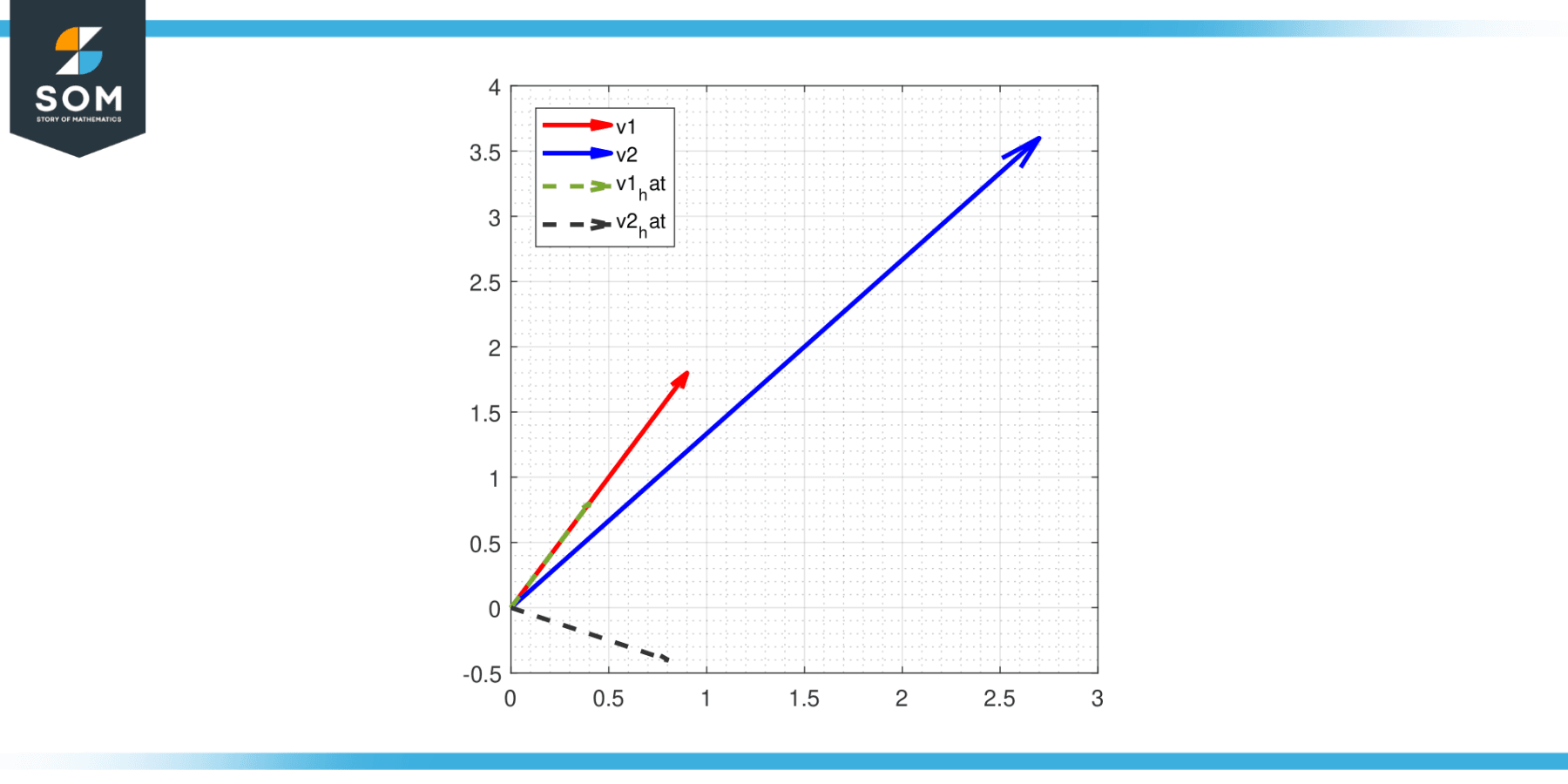
Figure-1.
The Gram-Schmidt process is a simple yet powerful procedure used to orthogonalize vectors. It is crucial in many disciplines, including computer science, physics, and mathematics, anywhere the idea of orthogonality is significant.
Applications
The Gram-Schmidt Process is crucial in mathematics, physics, and engineering because it generates orthogonal and orthonormal bases. Here are a few specific applications:
Quantum Mechanics
In quantum mechanics, the Gram-Schmidt process is often used to construct orthonormal bases for Hilbert spaces. These bases are useful for describing quantum states. For example, when dealing with the quantum harmonic oscillator or in second quantization, it is often necessary to construct a basis of orthonormal states.
Linear Algebra
The transformation of a collection of linearly independent vectors into an orthonormal basis is one of the main uses of the Gram-Schmidt process in linear algebra. The method’s main goal is to achieve this. An orthonormal basis simplifies many mathematical computations and is essential to various algorithms and transformations in linear algebra.
Computer Graphics and Vision
In 3D computer graphics, orthonormal bases represent objects’ orientation and position in space. The Gram-Schmidt Process can be used to compute these bases.
Signal Processing
The Gram-Schmidt Process is used in signal processing to create a set of orthogonal signals from initial signals. These orthogonal signals are used to reduce interference between transmitted signals.
Machine Learning
In machine learning, particularly in Principal Component Analysis (PCA), the Gram-Schmidt Process is used to orthogonalize the principal components, which are then used for dimensionality reduction.
Numerical Methods
The Gram-Schmidt Process forms the basis of the classical Gram-Schmidt method for numerically solving ordinary differential equations.
Control Systems
In control systems engineering, the Gram-Schmidt process is used to orthogonalize and normalize system modes, aiding in the analysis and design of stable and controllable systems.
Robotics
In robotics, the Gram-Schmidt process is utilized for sensor calibration, motion planning, and robot localization tasks, enabling accurate perception and control in robot environments.
Camera Calibration and 3D Reconstruction
In computer vision, one of the key tasks is to reconstruct a 3D scene from 2D images. A prerequisite for this task is camera calibration, where we need to find the intrinsic and extrinsic parameters of the camera. The intrinsic parameters include the focal length and principal point, and the extrinsic parameters refer to the rotation and translation of the camera with respect to the world.
Given enough 2D-3D correspondences, we can estimate the camera projection matrix. The Gram-Schmidt process is used to orthogonalize this matrix, effectively performing a QR decomposition, which can then be used to extract the camera parameters.
Augmented Reality (AR) and Virtual Reality (VR)
In AR and VR applications, the Gram-Schmidt process can be used to compute the orientation of objects and users in real-time. This is crucial for maintaining a consistent and immersive experience.
Object Recognition
In object recognition, the Gram-Schmidt process is often used to create a feature space. The features of an object in an image can be represented as vectors in a high-dimensional space. These vectors often have a lot of redundancy, and the Gram-Schmidt process can be used to orthogonalize these vectors, effectively creating a basis for the feature space. This reduces the dimensionality of the feature space, making the process of object recognition more computationally efficient.
Cryptography
In lattice-based cryptography, the Gram-Schmidt process is used for problems related to finding short vectors and close vectors, which are hard problems that are the basis of some cryptographic systems.
Econometrics and Statistics
The Gram-Schmidt process is used in regression analysis for the least squares method. It can help remove multicollinearity in multiple regression, which is when predictors correlate with each other and the dependent variable.
The utility of the Gram-Schmidt Process across these diverse fields underscores its fundamental importance in theoretical and applied mathematics. In all of these applications, the primary advantage of the Gram-Schmidt process is its ability to construct an orthonormal basis, which simplifies calculations and helps to reduce complex problems to simpler ones.
Exercise
Example 1
Let’s start with two vectors in R³:
v₁ = [1, 1, 1]
v₂ = [1, 2, 3]
We aim to construct an orthogonal basis for the subspace spanned by these vectors.
Step 1
We set the first vector of our new set to be u₁ = v₁:
u₁ = v₁ = [1, 1, 1]
Step 2
Compute the projection of v₂ onto u₁:
proj_u₁(v₂) = ((v₂ . u₁) / ||u₁||²) * u₁
proj_u₁(v₂) = (([1, 2, 3] . [1, 1, 1]) / ||[1, 1, 1]||²) * [1, 1, 1]
proj_u₁(v₂) = (6 / 3) * [1, 1, 1]
proj_u₁(v₂) = [2, 2, 2]
Subtract the projection from v₂ to obtain u₂:
u₂ = v₂ – proj_u₁(v₂)
u₂ = [1, 2, 3] – [2, 2, 2]
u₂ = [-1, 0, 1]
So, our orthogonal basis is {u₁, u₂} = {[1, 1, 1], [-1, 0, 1]}.
Example 2
Now, consider a case in R² with vectors:
v₁ = [3, 1]
v₂ = [2, 2]
Step 1
Begin with u₁ = v₁:
u₁ = v₁ = [3, 1]
Step 2
Compute the projection of v₂ onto u₁:
proj_u₁(v₂) = ((v₂ . u₁) / ||u₁||²) * u₁
proj_u₁(v₂) = (([2, 2] . [3, 1]) / ||[3, 1]||²) * [3, 1]
proj_u₁(v₂) = (8 / 10) * [3, 1]
proj_u₁(v₂) = [2.4, 0.8]
Subtract the projection from v₂ to obtain u₂:
u₂ = v₂ – proj_u₁(v₂)
u₂ = [2, 2] – [2.4, 0.8]
u₂ = [-0.4, 1.2]
Our resulting orthogonal basis is {u₁, u₂} = {[3, 1], [-0.4, 1.2]}.
All figures are generated using MATLAB.