
To graph a cosine function, I first set up a standard coordinate plane. On this plane, the horizontal axis (x-axis) represents the angle in radians, ranging from (0) to $2\pi$, and the vertical axis (y-axis) corresponds to the value of the cosine function, which varies between (-1) and (1).
Since the cosine function is periodic with a period of $2\pi$, its graph repeats every $2\pi$ unit along the x-axis. The shape of the cosine curve is wave-like and starts at a maximum value of (1) when the angle is (0) radians.
Graphing the cosine function requires plotting points that represent the angle and the cosine of that angle, and then connecting these points with a smooth curve.
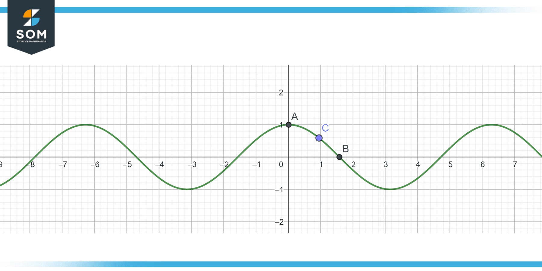
The curve peaks at (1) for $\cos(0)$ and $\cos(2\pi)$, dips to (-1) at $\cos(\pi)$, and intersects the x-axis at $\cos(\frac{\pi}{2})$ and $\cos(\frac{3\pi}{2})$.
Graphing the Cosine Functions
When I graph the cosine function, I start by recalling that it’s a trigonometric function known for its periodic nature.
The classic form of the cosine function can be expressed as $y = \cos(x) $, showcasing a wave that repeats every $2\pi$ radian. The amplitude, or the peak height from the center line, is 1, and the range of the cosine function is from -1 to 1.
The first step in graphing a cosine function is to set up my coordinate axes. The domain of the cosine is all real numbers, which means I need to consider how much of the x-axis I want to display.
Since it’s periodic, displaying one or two periods is often sufficient. For the classic cosine wave with $y = \cos(x)$, I mark key points at ( (0, 1) ), $ (\pi/2, 0) $, $(\pi, -1) $, $ (3\pi/2, 0) $, and $(2\pi, 1)$.
Sometimes, I encounter variations of the cosine function, like $y = A \cos(B(x – C)) + D$, where ( A ) is the amplitude, ( B ) affects the period, and ( C ) and ( D ) describe the horizontal (phase shift) and vertical shifts, respectively.
The period is given by $\frac{2\pi}{|B|}$. So, when B is greater than 1, the function compresses, and when B is less than 1, it stretches.
To make it clearer, here’s how the properties of cosine affect its graph:
| Property | Effect on Graph |
|---|---|
| Amplitude | Determines the height of peaks and depths of troughs |
| Period | The distance required for the function to complete one cycle |
| Phase shift | Moves the graph left or right |
| Vertical shift | Shifts the graph up or down |
Remember, to create an accurate graph, I pay close attention to these values and use proper scaling on my axes. By understanding these fundamentals, graphing any cosine function becomes a manageable task.
Advanced Concepts in Graphing Cosine
When I explore cosine graphs, I appreciate that they showcase unique characteristics indicative of even functions. The cosine function is the mirror image of itself across the y-axis, exhibiting symmetry about the y-axis.
While graphing, I consider this property, which tells me that the cosine function, $\cos(x) $, satisfies the condition $\cos(x) = \cos(-x)$.
As for the wave properties, I’m attentive to the fact that cosine and sine are sinusoidal functions. They share a period that I can determine by the formula $T = \frac{2\pi}{|k|}$, where ( k ) is the horizontal stretch factor.
They form a repeating pattern where cosine has its local maxima at the start ( (1, 0) ) on the unit circle and then oscillates to its local minima. Understanding the vertical stretch factor ( A ) is also essential; it modifies amplitude, affecting the maximum value to ( A ) and minimum value to ( -A ).
For graphing sine and cosine functions, I often sketch them together to compare their shapes. A graph of the cosine function generally starts at a maximum value, while the sine graph starts at the midline. This distinction becomes clear when I create a table of values or use an app to generate accurate graphs.
Here’s a succinct table noting key transformation traits for cosine:
| Transformation | Effect on $\cos(x)$ |
|---|---|
| Horizontal shift | Translates the wave along the x-axis |
| Horizontal stretch/compression | Alters the period of the wave |
| Vertical stretch | Modifies the amplitude of the wave |
| Reflection | Flips the graph over the x-axis or y-axis |
In pre-calculus and calculus, my studies include these advanced manipulations of the cosine graph on the coordinate plane. Whether it’s in radians or degrees, precisely determining the transformations allows me to sketch an accurate representation of my trigonometric function.
Conclusion
I’ve discussed the steps to graph the cosine function, illustrating its periodic nature and symmetry around the y-axis. Remember that the cosine function varies between $-1$ and $1$, and its graph is a wave that repeats every $2\pi$ radians.
I hope that my explanation has made it easier for you to grasp the procedure and plot the function accurately.
When you’re working on this, pay close attention to identifying the amplitude, period, phase shift, and vertical shift, as these will dictate the shape and position of your graph on the coordinate plane.
For the standard cosine function, $y = \cos(x)$, you’ll have an amplitude of $1$, no phase shift, no vertical shift, and a period of $2\pi$.
If you want to experiment, try altering these values to see how the graph changes. For example, a cosine function like $y = A \cos(Bx – C) + D$ can have a different look based on the values of $A$, $B$, $C$, and $D$.
But as long as you rely on the foundation I’ve shared, you’ll be able to tackle these variations confidently.
I’m glad I could walk you through the process of graphing a cosine function. With practice, I’m sure you’ll become comfortable with these concepts and apply them effectively in your work.