JUMP TO TOPIC

To sketch the graph of a function, I first consider the type of function and its features, such as intercepts, slopes, and asymptotes.
Drawing the graph of a function is a practical way to visualize the behavior of mathematical expressions over a given domain.
When I analyze the graph of a function, I look for key information that indicates how the function behaves across different intervals. This includes finding the zeros, the increases and decreases, and any points of discontinuity.
My strategy involves plotting known points, particularly where the function intersects the axes. For functions like polynomials, this may involve solving for when the function equals zero.
I then determine the interval over which I’m interested in the function’s behavior, whether it’s a specific range or a broader perspective.
Finally, I check for symmetry and other patterns that might simplify my sketch, ensuring my graph is comprehensive and accurate. By approaching the sketch methodically and considering these elements, I gain a complete picture of the function’s characteristics.
Steps Involved in Sketching Graph of a Function
When I begin to sketch the graph of a function, I first consider its domain and range.
The domain represents all possible input values (usually the x-values), which are the real numbers that can be plugged into the function without causing any undefined behavior.
For example, in the function $f(x) =2x-1$, the domain excludes the value $x = 1$ because it would make the denominator zero, which is undefined.
I then locate any asymptotes, which are lines the graph approaches but never touches. Vertical asymptotes often occur where the denominator of a rational function is zero, and horizontal asymptotes are linked to the behavior of the function as $x$ approaches infinity.
The slope of the function helps me understand how steep the graph is. For a linear function, the slope is constant, while for non-linear functions, the slope changes as $x$ changes.
When graphing, I use transformations such as reflection, shift, or stretching to adjust the basic graph of the function. A graphing calculator can be extremely helpful in this process, offering a visual representation of the function.
Identifying any critical points, such as local maxima and minima, and inflection points where the concavity changes, is also important. They give me detailed information about the function‘s behavior and help refine my sketch.
Here’s a quick reference table summarizing the steps:
| Step | Description |
|---|---|
| Domain and Range | Determine acceptable x and y values |
| Y-intercept | Set $x = 0$ in the equation |
| X-intercepts | Solve $f(x) = 0$ |
| Asymptotes | Look for values that make the function undefined |
| Slope and Curvature | Analyze slope changes to plot the curve |
| Transformations | Apply shifts and reflections to alter the basic graph |
| Critical Points | Find and plot maxima, minima, and inflection points |
With these steps, I’m equipped to create an accurate and detailed graph of most functions.
Exploring Sketch Features
When I begin sketching a graph, I find it immensely helpful to identify the essential characteristics of a function. These features help predict the appearance of the graph before I even put pen to paper.
Intervals of increase and decrease inform me about the slope of a function. In parts where a function is increasing, the graph moves upward as it goes from left to right, and when it’s decreasing, it slopes downward.
The points where a graph changes from increasing to decreasing or vice versa are known as critical points. These points often correspond to local extrema, which are the highs and lows of the graph.
Inflection points are also key: They are where the graph changes concavity, shifting between concave up (shaped like a cup) and concave down (shaped like a cap). ‘
A concise way to remember is that when a graph is concave up, the derivative is increasing, and when it’s concave down, the derivative is decreasing.
Finally, a snapshot of the end behavior can be taken by looking at what happens to the graph as ( x ) approaches infinity or negative infinity. Does it level off, or does it escape off to infinity? The answers give clues to the tails of the graph.
Here’s a quick reference table summarizing these features:
| Feature | Description | Impact on Graph |
|---|---|---|
| Intervals of Increase/Decrease | Regions where the function’s slope is positive/negative | Slope direction |
| Critical Points | Where the first derivative is zero or undefined | Potential local extrema |
| The Inflection Points | Where concavity changes | Slope curvature change |
| End Behavior | As ( x ) approaches ( \pm \infty ) | Tail direction |
By meticulously analyzing these characteristics, I can sketch a more accurate representation of any function.
Function Types and Characteristics
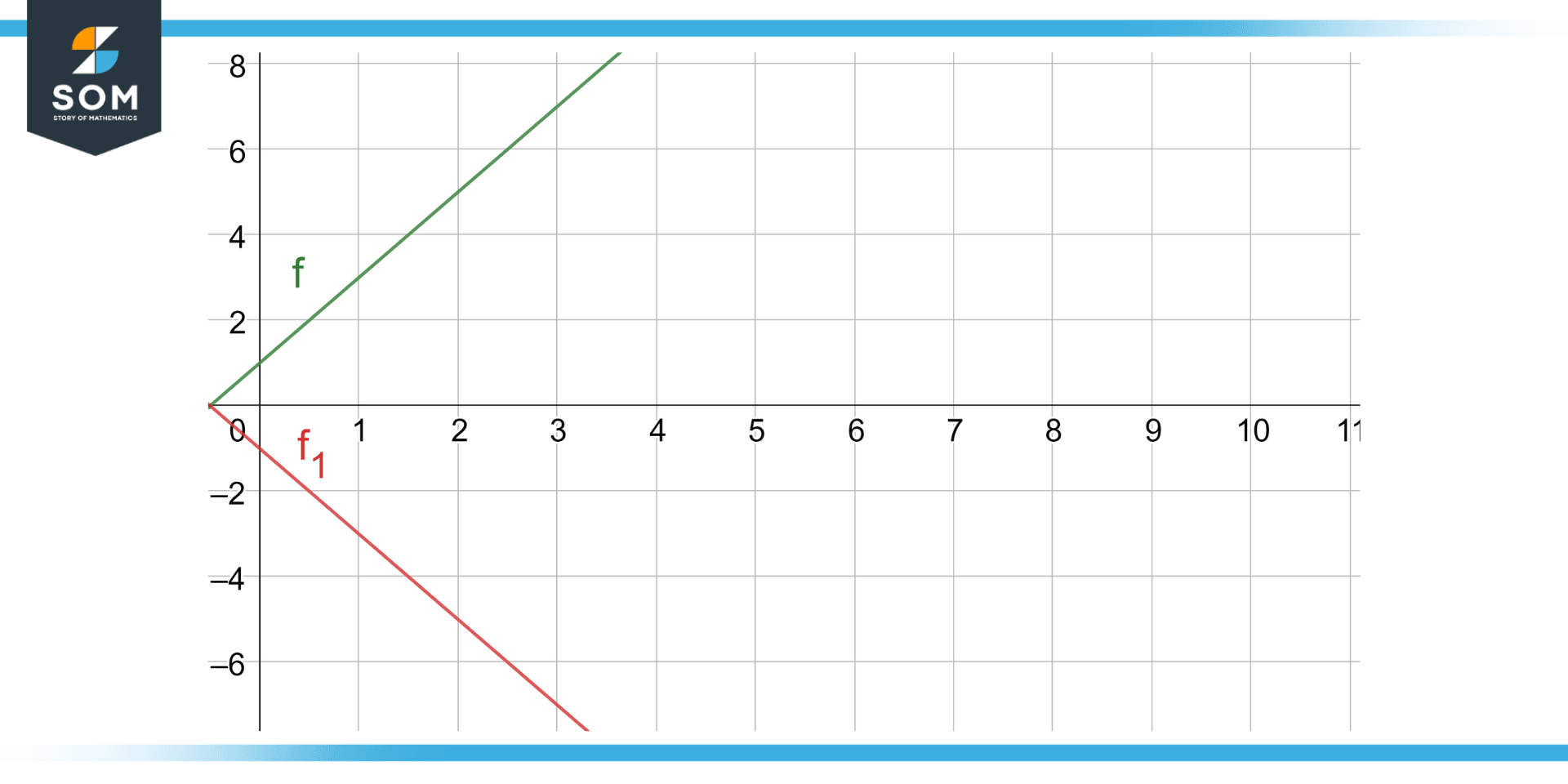
When I explore different types of functions, I first understand their characteristics and behavior. For instance, a linear function like ( f(x) = mx + b ) has a constant rate of change, known as the slope ( m ), and a y-intercept ( b ).
The graph is a straight line with slope ( m ) and y-intercept ( b ).
Moving on to polynomial functions, these can be expressed in the form $ f(x) = a_n x^n + a_{n-1} x^{n-1} + … + a_1 x + a_0 $, where ( n ) is the degree of the polynomial.
Notably, if ( n ) is even, the polynomial function can have a similar end behavior on both sides, while an odd-degree polynomial tends to have opposite end behaviors. Rational functions are formed by the quotient of two polynomials, like $ f(x) = \frac{p(x)}{q(x)} $.
They may have horizontal asymptotes, which I locate by comparing the degrees of the numerator and denominator polynomials. When the degree of the numerator is less than the denominator, the x-axis (y = 0) is typically the horizontal asymptote.
Transcendental functions include exponential, logarithmic, and trigonometric functions. These do not have a degree like polynomials but have their unique properties. For example, the exponential function $f(x) = e^x$ grows rapidly, and its derivative is itself.
To determine the nature of turning points or concavity, I utilize the first and second derivative tests.
Through the derivative, I identify critical points and use the second derivative to determine if the function is concave up (positive second derivative) or concave down (negative second derivative).
| Type | Definition | Characteristics |
|---|---|---|
| Linear | $f(x) = mx + b$ | Constant rate of change, straight line graph |
| Polynomial | $ f(x) = a_n x^n + … + a_0$ | Degree determines end behavior |
| Rational | $f(x) = \frac{p(x)}{q(x)}$ | May have horizontal asymptotes |
| Transcendental | $f(x) = e^x$ , etc. | Unique properties, not defined by a degree |
In summary, understanding these characteristics helps me sketch the curves accurately, predict their behavior, and analyze their properties more effectively.
Conclusion
In this guide, I’ve walked you through the steps to sketch the graph of a function efficiently. Remember, practice makes perfect.
The more functions you graph, the better intuition you’ll develop for their behavior. Use the domain, intercepts, and end behavior to establish a framework for your graph.
Techniques such as testing for even, odd, or periodic properties can simplify your work by revealing symmetries.
Always start with a clear understanding of the domain of your function, which reveals the possible x-values you can input. The intercepts give you specific points where the graph crosses the axes, with the x-intercepts found by solving the equation ( f(x) = 0 ) and the y-intercept by evaluating ( f(0) ).
For the end behavior, investigate the limits as ( x ) approaches infinity and negative infinity to determine horizontal asymptotes, if they exist. If a function approaches a particular y-value ( L ) as ( x ) grows large, you can denote this with a horizontal line ( y = L ).
By following these methods, I hope you feel more confident in your graphing skills. Keep your pencil moving, and look for patterns and relationships in the functions you plot.