JUMP TO TOPIC

Welcome to an engaging exploration of the Wronskian, an indispensable mathematical tool with profound applications. In this article, we embark on a journey to understand the intricacies and significance of the Wronskian.
Defined as a determinant formed from a set of functions, the Wronskian serves as a powerful tool for analyzing relationships, testing linear dependence, and revealing the solutions to differential equations.
Through an in-depth exploration of its calculations, properties, and practical applications, we will unlock the true potential of the Wronskian and witness its transformative impact on mathematical analysis. Join us as we delve into the fascinating world of the Wronskian and discover its remarkable contributions to the realm of mathematics.
Definition
Diving deep into the world of mathematics, one is bound to encounter a variety of intricate concepts, each with its unique significance and application. Among these is the Wronskian, a mathematical determinant that plays a pivotal role in the study and solution of differential equations.
This determinant, named after the renowned Polish mathematician Józef Hoene-Wroński, serves as a powerful tool to gauge the linear independence of solution sets.
By its definition, the Wronskian of two or more functions calculates the determinant of a specific kind of matrix. Each row of this matrix represents a progressively higher derivative of each function. By evaluating the determinant, we obtain a measure that helps decipher the relationship between the functions.
In the context of differential equations, the Wronskian determinant unveils crucial insights about solutions and their relationships. Specifically, it allows us to examine if a set of solutions to a differential equation are linearly independent – a critical piece of information when constructing the general solution. Below, we present an example of how the dependency of two generic functions can be identified by Wronskian.
Compute the Wronskian W(f, g) of the two simple functions f(x) and g(x) as given: f(x) = x and g(x) = x²
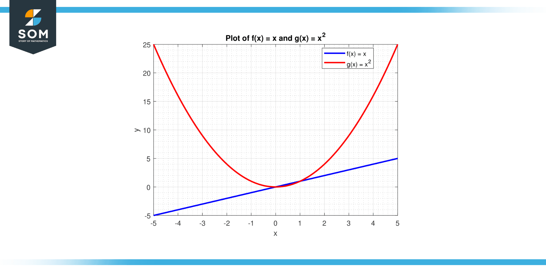
Figure-1.
The Wronskian W(f, g) is given by the determinant of a 2×2 matrix:
W(f, g) = det |f(x), g(x)|
W(f, g) = |f'(x), g'(x)|
This equates to:
W(f, g) = det |x, x²| |1, 2x|
The determinant of this matrix is:
W(f, g) = x*(2x) – (x²)*1
W(f, g) = 2x² – x²
W(f, g) = x²
Here, the Wronskian is zero only when x=0. Therefore, the functions f(x) and g(x) are linearly independent for x ≠ 0.
Historical Significance of Wronskian
The historical background of the Wronskian traces back to the 18th century, named after the Russian mathematician Nikolai Ivanovich Wronski (also spelled Vronsky or Wronskij). Born in 1778, Wronski made significant contributions to various branches of mathematics, including analysis, differential equations, and algebra. However, it is worth noting that the concept of the Wronskian predates Wronski’s work, with earlier developments by mathematicians such as Jean le Rond d’Alembert and Joseph-Louis Lagrange.
Wronski’s interest in the Wronskian emerged in his investigations of differential equations and the theory of linear dependence. He recognized the value of a determinant formed from a set of functions in analyzing the linear independence of solutions to differential equations. Wronski’s work on the Wronskian led to the development of its properties and applications, solidifying its importance as a mathematical tool.
While Wronski’s contributions were significant, the use of determinants in the context of linear dependence and differential equations can be traced back even further to mathematicians like Carl Jacobi and Augustin-Louis Cauchy. They explored related concepts and techniques that laid the foundation for the subsequent developments in the theory of determinants and the Wronskian.
Today, the Wronskian continues to be a central tool in mathematical analysis, playing a crucial role in various fields such as differential equations, linear algebra, and mathematical physics. Its historical development showcases the collaborative efforts and contributions of mathematicians over time, paving the way for its applications and a deeper understanding of functions, dependencies, and differential equations.
Properties of Wronskian
The Wronskian, being a significant tool in the field of differential equations, has several important properties and characteristics which govern its behavior and utility. Below are the fundamental properties associated with the Wronskian:
Linearity in Each Argument
The Wronskian exhibits linearity, meaning that it satisfies the property of being linear with respect to its component functions. Specifically, if W(f₁, f₂, …, fₙ) is the Wronskian of a set of functions, and a₁, a₂, …, aₙ are constants, then the Wronskian of the linear combination a₁f₁ + a₂f₂ + … + aₙfₙ is equal to a₁W(f₁, f₂, …, fₙ) + a₂W(f₁, f₂, …, fₙ) + … + aₙW(f₁, f₂, …, fₙ).
Nonzero Wronskian Implies Linear Independence
If the Wronskian of a set of functions is nonzero for at least one value in an interval, then those functions are linearly independent on that interval. This is an important and often-used property in the study of differential equations.
Zero Wronskian Does Not Necessarily Imply Linear Dependence
A crucial subtlety of the Wronskian is that a zero value does not necessarily indicate linear dependence. This is contrary to the intuition one might have from linear algebra, where a zero determinant signifies linear dependence. In the context of functions, there exist sets of functions that are linearly independent yet have a zero Wronskian.
Wronskian of Solutions to a Linear Homogeneous Differential Equation
If we have a set of solutions to a linear homogeneous differential equation, then either the Wronskian of these solutions is identically zero for all x in the interval, or it is never zero. This result ties in closely with the second and third properties. It essentially means that for solutions to a linear homogeneous differential equation, a zero Wronskian does indicate linear dependence.
Wronskian and the Existence of Solutions
The Wronskian can provide information about the existence of solutions to a linear differential equation. If the Wronskian is non-zero at a point, then there exists a unique solution to the linear differential equation that satisfies given initial conditions at that point.
Abel’s Identity/Theorem
This theorem gives a relationship for how the Wronskian of solutions to a second-order linear homogeneous differential equation changes. Specifically, it shows that the Wronskian either is always zero or always non-zero, depending on whether the solutions are linearly dependent or independent.
Related Formulas
The Wronskian is a determinant used in the study of differential equations, particularly to determine whether a set of solutions is linearly independent. Here are the key related formulas:
Wronskian of Two Functions
For two differentiable functions f(x) and g(x), the Wronskian is given by:
W(f, g) = det |f(x), g(x)|
W(f, g) = |f'(x), g'(x)|
The vertical bars |…| denote a determinant. This evaluates to:
W(f, g) = f(x) * g'(x) – g(x) * f'(x)
Wronskian of Three Functions
For three differentiable functions f(x), g(x), and h(x), the Wronskian is given by the determinant of a 3×3 matrix as given below:
W(f, g, h) = det |f(x), g(x), h(x)|
W(f, g, h) = |f'(x), g'(x), h'(x)|
W(f, g, h) = |f”(x), g”(x), h”(x)|
Wronskian of n Functions
When you are dealing with n functions, the Wronskian is a determinant of an n x n matrix. The Wronskian for n functions, {f₁(x), f₂(x), …, fₙ(x)}, is defined as follows:
W(f₁, f₂, …, fₙ)(x) = det |f₁(x), f₂(x), …, fₙ(x)|
W(f₁, f₂, …, fₙ)(x) = |f₁'(x), f₂'(x), …, fₙ'(x)|
|… , …, …, …|
W(f₁, f₂, …, fₙ)(x) = | f₁⁽ⁿ⁻¹⁾(x) f₂⁽ⁿ⁻¹⁾(x) … fₙ⁽ⁿ⁻¹⁾(x) |
Here’s what each part of this formula means:
f₁(x), f₂(x), …, fₙ(x) are the functions under consideration.
f₁'(x), f₂'(x), …, fₙ'(x) are the first derivatives of the functions.
f₁⁽ⁿ⁻¹⁾(x) f₂⁽ⁿ⁻¹⁾(x) … fₙ⁽ⁿ⁻¹⁾(x) are the (n-1)-th derivatives of the functions.
The Wronskian is thus a square matrix with n rows and n columns. Each row represents a different order of derivatives, from 0 (the original functions) up to the (n-1)-th derivative. The determinant of this matrix is then computed in the standard way for determinants of square matrices.
Abel’s Identity/Theorem
This gives a relationship for how the Wronskian of solutions to a second-order linear homogeneous differential equation changes. Specifically, if y1 and y2 are solutions to the differential equation y” + p(x)y’ + q(x)y = 0, then their Wronskian W(y1, y2) satisfies the equation:
d/dx [W(y1, y2)] = -p(x) * W(y1, y2)
These formulas are the backbone of the Wronskian concept. They allow us to calculate the Wronskian for any set of differentiable functions and hence test for linear independence. In particular, Abel’s Identity provides crucial information about the behavior of the Wronskian for solutions to second-order linear homogeneous differential equations.
Calculation Technique
The Wronskian calculation technique involves determining the determinant of a specific type of matrix where each row is a progressively higher derivative of each function. This technique is primarily used to assess the linear independence of a set of functions.
Set of Functions
Begin with a set of functions, denoted as f₁(x), f₂(x), …, fₙ(x), where x represents the independent variable.
Two Functions
Let’s start with the Wronskian for two functions, f and g. The Wronskian is given by W(f, g) = f(x) * g'(x) – g(x) * f'(x). This involves taking the derivative of each function and calculating the difference of the products of functions and their derivatives.
Three Functions
If we have three functions, f, g, and h, the Wronskian becomes a 3×3 determinant. Here’s the format:
W(f, g, h) = det |f(x), g(x), h(x)|
W(f, g, h) = |f'(x), g'(x), h'(x)|
W(f, g, h) = |f”(x), g”(x), h”(x)|
More than Three Functions
If we have more than three functions, the method generalizes in the same way: you form a square matrix where the i-th row is the (i-1)th derivative of each function and then compute the determinant.
Order of Derivatives
In the above matrices, the first row is the 0th derivative (i.e., the functions themselves), the second row is the first derivative, the third row is the second derivative, and so on.
Construct the Matrix
Create an n x n matrix, where n is the number of functions in the set. The matrix will have n rows and n columns.
Matrix Entries
Assign the derivatives of the functions as entries to the matrix. Each entry aᵢⱼ corresponds to the derivative of function fⱼ(x) with respect to x, evaluated at a particular point. In other words, aᵢⱼ = fⱼ⁽ⁱ⁾(x₀), where fⱼ⁽ⁱ⁾(x₀) denotes the i-th derivative of function fⱼ(x) evaluated at x₀.
Matrix Formation
Arrange the entries in the matrix, following a specific pattern. The i-th row of the matrix corresponds to the derivatives of each function evaluated at the same point x₀.
Calculate the Determinant
Evaluate the determinant of the constructed matrix. This can be done using various methods, such as expanding along a row or column or applying row operations to transform the matrix into an upper triangular form.
Simplify and Interpret
Simplify the determinant expression if possible, which may involve algebraic manipulations and simplification techniques. The resulting expression represents the value of the Wronskian for the given set of functions.
It is important to note that the specific form and complexity of the Wronskian calculation may vary depending on the functions involved and the desired level of detail. In some cases, the functions may have explicit formulas, making it easier to calculate their derivatives and form the matrix. In other situations, numerical or computational methods may be employed to approximate the Wronskian.
By performing the Wronskian calculation, mathematicians and scientists gain insights into the linear dependence or independence of functions, the behavior of solutions to differential equations, and other mathematical properties associated with the given set of functions.
Evaluating Linear Dependence/Independence using Wronskians
Wronskian is often used to evaluate whether a given set of functions are linearly dependent or linearly independent. This is especially important when solving differential equations, as knowing the linear independence of solutions can be quite insightful. To understand this better, let’s first define what linear dependence and independence mean:
A set of functions {f₁(x), f₂(x), …, fₙ(x)} is said to be linearly independent on an interval I if no nontrivial linear combination of them is identically zero on that interval. In other words, there are no constants c₁, c₂, …, cₙ (not all zero) such that c₁f₁(x) + c₂f₂(x) + … + cₙfₙ(x) = 0 for all x in I. Conversely, if such a nontrivial linear combination exists, the functions are said to be linearly dependent.
When it comes to using the Wronskian to evaluate these properties, the following principles apply:
If the Wronskian W(f₁, f₂, …, fₙ) of a set of functions is nonzero at a point within the interval I, the functions are linearly independent on that interval.
If the Wronskian is identically zero on the interval I (that is, it’s zero for all x in I), the functions are linearly dependent.
However, one must be cautious: a zero Wronskian does not necessarily imply linear dependence. This is because there can be points or intervals where the Wronskian is zero while the functions are still linearly independent. Therefore, a nonzero Wronskian confirms linear independence, but a zero Wronskian doesn’t confirm linear dependence.
For higher-order differential equations, the Wronskian, combined with Abel’s Identity, can also be used to demonstrate the existence of a fundamental set of solutions and the uniqueness of solutions.
Applications
The Wronskian, named after the Polish mathematician Józef Hoene-Wroński, is a key tool in the mathematical study of differential equations. It serves as a test for the linear independence of a set of solutions to differential equations. Beyond its role in mathematics, the Wronskian has several applications in diverse fields.
Physics
In physics, particularly quantum mechanics, the Wronskian plays an indispensable role. In the realm of quantum physics, the Schrödinger equation, a fundamental differential equation, describes the quantum state of a physical system. The solutions to this equation, called wave functions, must be orthogonal (linearly independent), and the Wronskian can be employed to check their orthogonality. When solutions of the Schrödinger equation are sought, the Wronskian helps to confirm the linear independence of potential solutions and hence guarantees the validity of the physical model.
Engineering
The field of engineering also sees the application of the Wronskian, particularly in electrical and mechanical engineering domains. These fields often involve the study of complex systems modeled by systems of differential equations. In understanding the nature of these solutions, the Wronskian serves as an essential instrument. In system stability analysis and control theory, engineers use the Wronskian to identify the independent modes of a system described by linear differential equations. Furthermore, in vibration analysis of mechanical systems, linear independence of modes, ascertained by the Wronskian, is crucial.
Economics
In Economics, specifically, econometrics leverages the Wronskian as well. Economists often use differential equations to model complex dynamic systems, such as market equilibrium dynamics, economic growth models, and more. Assessing the linear independence of the solutions to these equations is crucial to ensure the validity of the model and its predictions. This is where the Wronskian finds its use.
Computer Science
In computer science, especially in machine learning and artificial intelligence, understanding the linear independence of functions can be essential. Even though the Wronskian itself might not be directly applied in this field, the concept it helps examine—linear independence—is significant. Particularly in feature selection for machine learning models, it’s important to select features (variables) that bring new, independent information to the model. This concept mirrors the mathematical idea of linear independence that Wronskian helps evaluate.
Numerical Analysis
The Wronskian also has implications in the realm of numerical analysis, a branch of mathematics concerned with devising algorithms for the practical approximation of solutions to mathematical problems. The Wronskian can be used to determine the accuracy of numerical solutions to differential equations. By examining the Wronskian of the numerically approximated solutions, we can check whether the solutions maintain their linear independence, which is crucial for confirming the correctness of the numerical methods used.
Education
In the field of education, particularly in advanced mathematics and physics courses, the Wronskian is a fundamental concept that educators teach to students to equip them with the skills to solve differential equations and to understand the concept of linear independence of functions. This concept is foundational in these fields and many others, so its understanding is fundamental to students.
Differential Equations
One of the primary applications of the Wronskian is in the field of differential equations. Differential equations are equations involving derivatives and are fundamental in modeling various phenomena in science and engineering. The Wronskian plays a crucial role in determining the linear independence of solutions to homogeneous linear differential equations.
Consider a homogeneous linear differential equation of the form:
aₙ(x)yⁿ + aₙ₋₁(x)yⁿ⁻¹ + … + a₁(x)y’ + a₀(x)y = 0
where y is the unknown function and a₀(x), a₁(x), …, aₙ(x) are continuous functions of x. If we have a set of n solutions y₁(x), y₂(x), …, yₙ(x), the Wronskian of these solutions is defined as:
W(y₁, y₂, …, yₙ)(x) = | y₁(x) y₂(x) … yₙ(x) |
W(y₁, y₂, …, yₙ)(x) = | y₁'(x) y₂'(x) … yₙ'(x) |
| … |
W(y₁, y₂, …, yₙ)(x) = | y₁⁽ⁿ⁻¹⁾(x) y₂⁽ⁿ⁻¹⁾(x) … yₙ⁽ⁿ⁻¹⁾(x) |
where y’ represents the derivative of y with respect to x, and y⁽ⁿ⁻¹⁾ denotes the (n-1)-th derivative of y.
The Wronskian can provide essential information about the linear dependence or independence of the solutions. If the Wronskian is nonzero for a particular value of x (or for a range of values), then the solutions y₁, y₂, …, yₙ are linearly independent over that interval. Conversely, if the Wronskian is identically zero for all x in an interval, the solutions are linearly dependent.
This property of the Wronskian is invaluable in determining the existence of linearly independent solutions to differential equations and establishing fundamental concepts in the theory of differential equations.
Function Analysis
The Wronskian is employed in function analysis to study the behavior and properties of functions. It is particularly useful in analyzing sets of functions and their relationships. By examining the Wronskian, mathematicians can determine the linear independence or dependence of functions, which is crucial for understanding the underlying structure and properties of the system.
Quantum Mechanics
The Wronskian finds applications in quantum mechanics, specifically in the study of wave functions. It is employed to determine the normalization of wave functions, which ensures that the probability density remains meaningful and satisfies certain conditions.
Despite its seemingly complex nature, the Wronskian is an incredibly versatile tool with a broad range of applications in various fields. Its ability to discern the nature of solutions to differential equations is an invaluable asset that helps simplify and solve otherwise complex systems.
Whether in quantum physics or economics, control theory or machine learning, the Wronskian stands as a testament to the wide-reaching applicability of mathematical concepts.
Exercise
Example 1
Compute the Wronskian W(f, g) of the two functions f(x) and g(x) as given in Figure-1.
$$f(x) = e^{x}$$
and
$$g(x) = e^{-x}$$
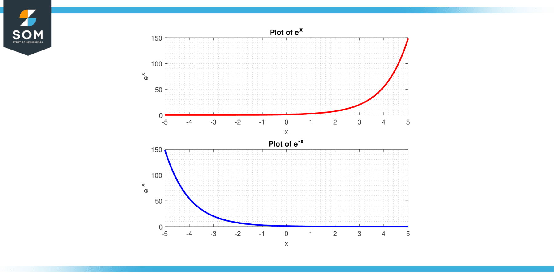
Figure-2.
Solution
Their Wronskian W(f, g) will be:
W(f, g) = det |f(x), g(x)|
W(f, g) = |f'(x), g'(x)|
This gives us:
$$W(f, g) = \det \begin{vmatrix} e^x & x \cdot e^x \end{vmatrix}$$
$$W(f, g) = \det \begin{vmatrix} e^x & e^x + x \cdot e^x \end{vmatrix}$$
Calculating the determinant, we get:
$$W(f, g) = e^x (e^x + x \cdot e^x) – (x e^x e^x) $$
$$W(f, g) = e^x $$
In this case, the Wronskian is always non-zero for any real x, hence the functions f(x) and g(x) are linearly independent.
Example 2
Compute the Wronskian W(f, g, h) of the three functions f(x), g(x) and h(x) as given:
f(x) = 1
g(x) = x
and
h(x) = x²
Solution
Their Wronskian W(f, g, h) will be the determinant of a 3×3 matrix:
W(f, g, h) = det |f(x), g(x), h(x)|
W(f, g, h) = |f'(x), g'(x), h'(x)|
W(f, g, h) = |f”(x), g”(x), h”(x)|
This gives us:
W(f, g, h) = det |1, x, x²|
W(f, g, h) = |0, 1, 2x|
W(f, g, h) = |0, 0, 2|
Calculating this determinant, we get:
W(f, g, h) = 1 * (1 * 2 – 2x * 0) – x * (0 * 2 – 2x * 0) + x² * (0 * 0 – 1 * 0)
W(f, g, h) = 2
As the Wronskian is non-zero, these three functions are linearly independent.
Example 3
For thefunctions given in Figure-2, calculate their Wronskian W(f, g).
f(x) = sin(x)
g(x) = cos(x)
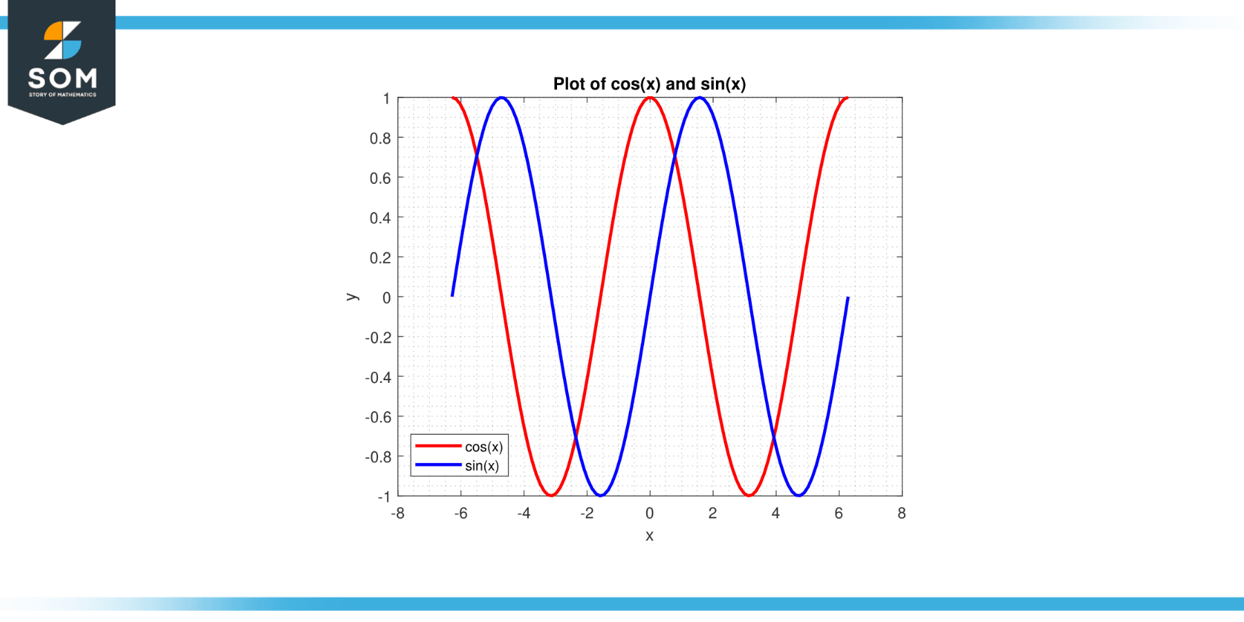
Figure-3.
Solution
Their Wronskian W(f, g) will be:
W(f, g) = det |f(x), g(x)|
W(f, g) = |f'(x), g'(x)|
This gives us:
W(f, g) = det |sin(x), cos(x)|
W(f, g) = |cos(x), -sin(x)|
Calculating the determinant, we get:
W(f, g) = sin(x) * (-sin(x)) – (cos(x) * cos(x))
W(f, g) = -sin²(x) – cos²(x)
W(f, g) = -1
As the Wronskian is non-zero for all x, the functions f(x) and g(x) are linearly independent.
Example 4
Let’s consider three functions: f(x) = x, g(x) = x², h(x) = x³, as given in Figure-3. Find the Wronskian W(f, g, h).
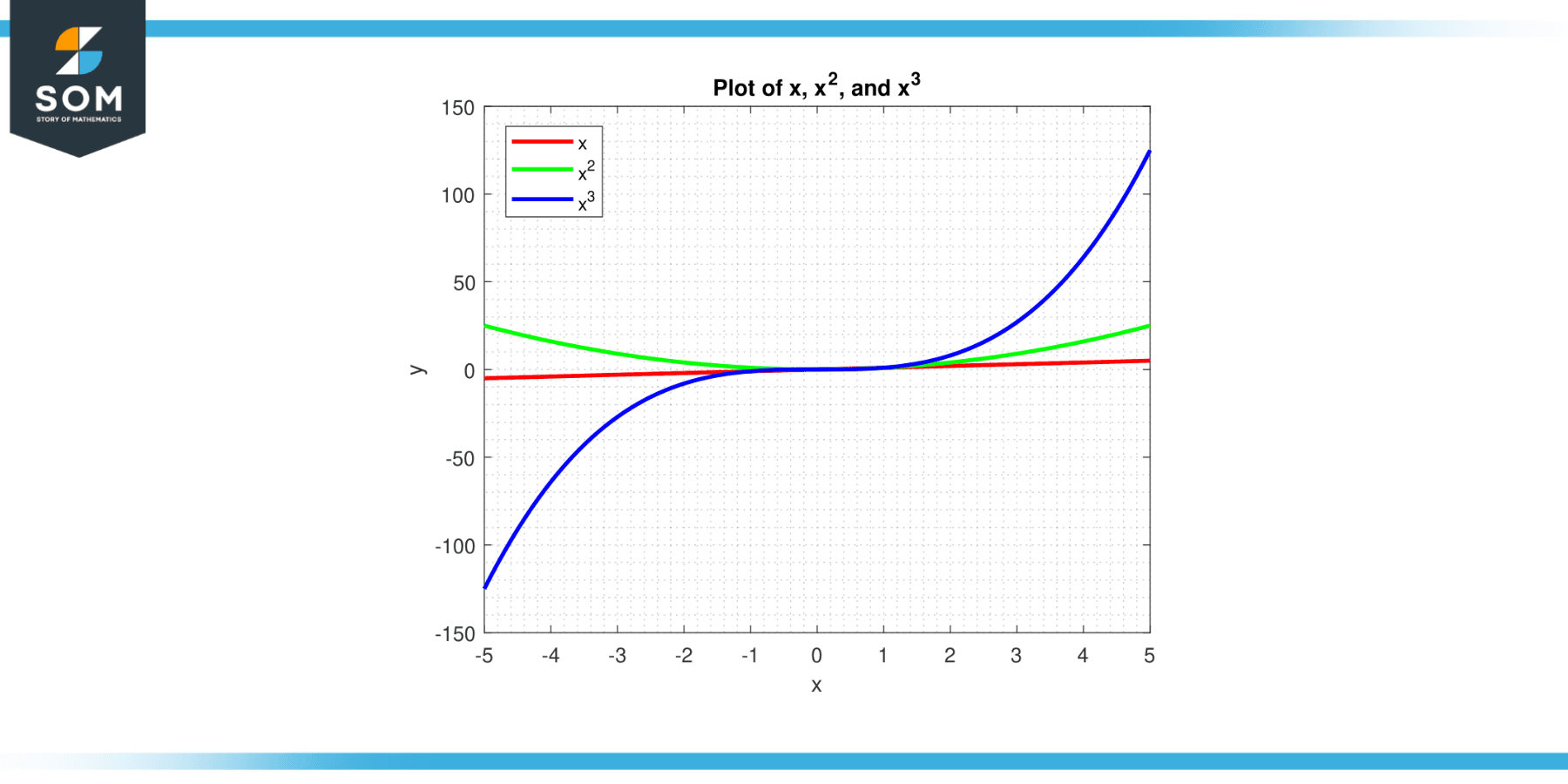
Figure-4.
Solution
Their Wronskian W(f, g, h) will be:
W(f, g, h) = det |f(x), g(x), h(x)|
W(f, g, h) = |f'(x), g'(x), h'(x)|
W(f, g, h) = |f”(x), g”(x), h”(x)|
This gives us:
W(f, g, h) = det |x, x², x³|
W(f, g, h) = |1, 2x, 3x²|
W(f, g, h) = |0, 2, 6x|
Calculating this determinant, we get:
W(f, g, h) = x * (2 * 6x – 3x² * 2) – x² * (1 * 6x – 3x² * 0) + x³ * (1 * 2 – 2x * 0)
W(f, g, h) = 12x² – 6x³
W(f, g, h) = 6x² (2 – x)
The Wronskian is zero when x = 0 or x = 2, and non-zero elsewhere. Hence, these three functions are not linearly independent for all x, but they are linearly independent for x ≠ 0, 2.
All figures are generated using MATLAB.