JUMP TO TOPIC
Bayes Theorem – Explanation & Examples
 The definition of the Bayes theorem is:
“Bayes theorem gives the probability of an event based on new information that is related to that event.”
In this topic, we will discuss the Bayes theorem from the following aspects:
- What is Bayes theorem?
- How to use the Bayes theorem?
- Tree diagrams.
- Bayes theorem formula.
- When to use Bayes theorem?
- Practice questions.
- Answer key.
1. What is Bayes theorem?
Bayes theorem gives the probability of an event based on new information that is related to that event.
Bayes theorem uses prior probability to generate posterior probability.
Prior probability is the probability of an event before new data is collected.
The posterior probability is the revised probability of an event after collecting new information. The posterior probability is calculated by updating the prior probability using the Bayes theorem.
For example, if the rate of a certain disease in a certain population is 0.1 or 10%.
This is the prior probability and it means that the probability or the risk of this disease for any individual from this population is 10%.
If this probability is known to increase with age, the Bayes theorem allows the risk of an individual (prior probability) to be updated to the more accurate posterior probability based on the individual’s age (new information).
Bayes theorem was named after the British mathematician Thomas Bayes.
2. How to use the Bayes theorem?
We will go through several examples.
– Example 1
A study in 1994 examined 491 dogs that had developed cancer and 945 dogs as a control group to determine whether there is an increased risk of cancer in dogs that are exposed to the herbicide 2,4-Dichlorophenoxyacetic acid (2,4-D).
Reference:
Hayes HM, Tarone RE, Cantor KP, Jessen CR, McCurnin DM, and Richardson RC. 1991. Case-Control Study of Canine Malignant Lymphoma: Positive Association With Dog Owner’s Use of 2, 4- Dichlorophenoxyacetic Acid Herbicides. Journal of the National Cancer Institute 83(17):1226-1231.
The results of this study are shown in the following table.
cancer | no cancer | Sum | |
2,4-D | 191 | 304 | 495 |
no 2,4-D | 300 | 641 | 941 |
Sum | 491 | 945 | 1436 |
The “cancer” and “no cancer” columns for dogs that developed and did not develop cancer respectively.
The “2,4-D” and “no 2,4-D” rows for dogs that were exposed and were not exposed to 2,4-Dichlorophenoxyacetic acid respectively.
We see that:
- 191 dogs that were exposed to 2,4-D developed cancer.
- 304 dogs that were exposed to 2,4-D did not develop cancer.
- 300 dogs that were not exposed to 2,4-D developed cancer.
- 641 dogs that were not exposed to 2,4-D did not develop cancer.
If we calculate the proportion (or probability) of each cell, we will get the following:
| cancer | no cancer | Sum |
2,4-D | 0.133 | 0.212 | 0.345 |
no 2,4-D | 0.209 | 0.446 | 0.655 |
Sum | 0.342 | 0.658 | 1.000 |
We see that:
- 0.13 or 13% of our data were dogs that were exposed to 2,4-D and developed cancer.
- 0.21 or 21% of our data were dogs that were exposed to 2,4-D and did not develop cancer.
- 0.21 or 21% of our data were dogs that were not exposed to 2,4-D and developed cancer.
- 0.45 or 45% of our data were dogs that were not exposed to 2,4-D and did not develop cancer.
We call these proportions or probabilities joint probabilities because they are for two variables (exposing to 2,4-D and developing cancer).
The sum probabilities are marginal probabilities because they are based on a single variable without regard to any other variable.
We see the following marginal probabilities in our data:
- 0.34 or 34% of our data were dogs that were exposed to 2,4-D = proportion of exposed dogs to 2,4-D that developed cancer + proportion of exposed dogs to 2,4-D that did not develop cancer = 0.13+0.21 = 0.34.
- 0.66 or 66% of our data were dogs that were not exposed to 2,4-D = proportion of non-exposed dogs to 2,4-D that developed cancer + proportion of non-exposed dogs to 2,4-D that did not develop cancer = 0.21+0.45 = 0.66.
- 0.34 or 34% of our data were dogs that developed cancer = proportion of cancer dogs that exposed to 2,4-D + proportion of cancer dogs that were not exposed to 2,4-D = 0.13+0.21 = 0.34.
- 0.66 or 66% of our data were dogs that did not develop cancer = proportion of non-cancerous dogs that were exposed to 2,4-D + proportion of non-cancerous dogs that were not exposed to 2,4-D = 0.21+0.45 = 0.66.
A third type of probability is called conditional probability because we compute this probability under a condition.
There are two parts of a conditional probability, the outcome of interest and the condition.
The condition is information or event that we know to be true. We separate the text inside our probability notation into the outcome of interest and the condition with a vertical bar.
If we consider the outcome of interest is developing cancer and the condition is exposing to 2,4-D.
The probability of developing cancer when the dog is exposed to 2,4-D =
p(developing cancer given that the dog is exposed to 2,4-D) =
p(developing cancer|exposed to 2,4-D) =
the number of dogs that developed cancer and exposed to 2,4-D / number of dogs that were exposed to 2,4-D = 191/495 = 0.39 or 39%.
If we have proportions, we can also calculate this conditional probability:
The probability of developing cancer when the dog is exposed to 2,4-D =
p(cancer|exposed to 2,4-D) =
The proportion of dogs that developed cancer and exposed to 2,4-D / proportion of dogs that were exposed to 2,4-D = 0.133/0.345 = 0.39 or 39%.
The probability of developing cancer for any dog is 0.342 or 34.2%. This is the prior probability or the marginal probability.
Knowing that the dog is exposed to 2,4-D increased its probability of developing cancer from 34% to 39%. The last probability is the posterior probability or the conditional probability.
The conditional probability of outcome A given condition B is computed as follows:
P(A|B)=(P(A and B))/(P(B))
Where P(A and B) = joint probability of A and B.
P(B) is the marginal probability of B.
The vertical bar “|” is read as given.
– Example 2
In the above example, calculate the probability of exposure to 2,4-D when the dog has cancer.
This is the inverse of the previous probability.
The probability of exposure to 2,4-D when the dog has cancer =
p(exposure to 2,4-D|cancer) =
Proportion of dogs that developed cancer and exposed to 2,4-D / proportion of dogs that have cancer = 0.133/0.342 = 0.39 or 39%.
The probability of 2,4-D exposure for any dog is 0.345 or 34.5%. This is the prior probability or the marginal probability.
Knowing that the dog has cancer increased its probability of being exposed to 2,4-D from 34.5% to 39%. The last probability is the posterior probability or the conditional probability.
– Example 3
A sample of 6,224 individuals from the year 1721 who were exposed to smallpox in Boston. Some of them had received a vaccine (inoculated) while others had not. Doctors at the time believed that inoculation, which involves exposing a person to the disease in a controlled form, could reduce the likelihood of death.
Reference:
Fenner F. 1988. Smallpox and Its Eradication (History of International Public Health, No. 6). Geneva: World Health Organization. ISBN 92-4-156110-6.
The results of this study are shown in the following table.
| no | yes | Sum |
died | 844 | 6 | 850 |
lived | 5136 | 238 | 5374 |
Sum | 5980 | 244 | 6224 |
The “no” and “yes” columns for persons who did not receive and received the vaccine respectively.
The “died” and “lived” rows for the died and lived persons.
We see that:
- 844 persons who did not receive the vaccine died.
- 5136 persons who did not receive the vaccine lived.
- 6 persons who received the vaccine died.
- 238 persons who received the vaccine lived.
If we calculate the proportion (or probability) of each cell, we will get the following:
| no | yes | Sum |
died | 0.136 | 0.001 | 0.137 |
lived | 0.825 | 0.038 | 0.863 |
Sum | 0.961 | 0.039 | 1.000 |
We see that:
- 0.136 or 13.6% of our data were persons who did not receive the vaccine and died.
- 0.825 or 82.5% of our data were persons who did not receive the vaccine and lived.
- 0.001 or 0.1% of our data were persons who received the vaccine and died.
- 0.038 or 3.8% of our data were persons who received the vaccine and lived.
We call these proportions or probabilities joint probabilities because they for two variables (receiving the vaccine and living).
The sum probabilities are marginal probabilities because they are based on a single variable without regard to any other variable.
We see the following marginal probabilities in our data:
- 0.961 or 96.1% of our data were persons that did not receive the vaccine = proportion of persons that did not receive the vaccine and died + proportion of persons that did not receive the vaccine and lived = 0.136+0.825 = 0.961.
- 0.039 or 3.9% of our data were persons who received the vaccine = proportion of persons who received the vaccine and died + persons who received the vaccine and lived = 0.001+0.038 = 0.039.
- 0.137 or 13.7% of our data were persons who died = proportion of persons who did not receive the vaccine and died + proportion of persons who received the vaccine and died = 0.136+0.001 = 0.137.
- 0.863 or 86.3% of our data were persons who lived = proportion of persons who did not receive the vaccine and lived + proportion of persons who received the vaccine and lived = 0.825+0.038 = 0.863.
We can calculate several conditional probabilities:
- The probability of person died from smallpox given that he was not inoculated= p(died|did not receive the vaccine) = p(died and did not receive the vaccine)/ p(did not receive the vaccine) = 0.136/0.961 = 0.142 or 14.2%.
The probability of dead persons is 0.137 or 13.7%. This is the prior probability or the marginal probability.
Knowing that the dead persons did not receive the vaccine increased its probability of dying from 13.7% to 14.2%. The last probability is the posterior probability or the conditional probability.
- The probability of person died from smallpox given that he was inoculated= p(died|received the vaccine) = p(died and received the vaccine)/ p(received the vaccine) = 0.001/0.039 = 0.026 or 2.6%.
The probability of dead persons is 0.137 or 13.7%. This is the prior probability or the marginal probability.
Knowing that the dead persons received the vaccine decreased his probability of dying from 13.7% to 2.6%. The last probability is the posterior probability or the conditional probability.
Comparing the two probabilities, the death rate for persons who were not inoculated is about (14.2/2.6 = 5.5) 5.5 times the death rate for persons who were inoculated or received the vaccine.
- The probability of person living from smallpox given that he was not inoculated= p(lived|did not receive the vaccine) = p(lived and did not receive the vaccine)/ p(did not receive the vaccine) = 0.825/0.961 = 0.858 or 85.8%.
The probability of lived persons is 0.863 or 86.3%. This is the prior probability or the marginal probability.
Knowing that the lived persons did not receive the vaccine decreased its probability of dying from 86.3% to 85.8%. The last probability is the posterior probability or the conditional probability.
- The probability of person lived from smallpox given that he was inoculated= p(lived|received the vaccine) = p(lived and received the vaccine)/ p(received the vaccine) = 0.038/0.039 = 0.974 or 97.4%.
The probability of lived persons is 0.863 or 86.3%. This is the prior probability or the marginal probability.
Knowing that the lived persons received the vaccine increased his probability of living from 86.3% to 97.4%. The last probability is the posterior probability or the conditional probability.
Comparing the two probabilities, the living rate for persons who were inoculated is about (97.4/85.8 = 1.1) 1.1 times the living rate for persons who were not inoculated or did not receive the vaccine.
3. Tree diagrams
Tree diagrams are a tool to organize outcomes and probabilities.
They are useful when two or more processes occur in a sequence and each process is conditioned on its predecessors.
The smallpox data fit this description. We see the population is split by inoculation: yes and no. Following this split, survival rates were observed for each group.
The following tree diagram shows these probabilities:
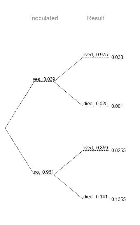
The first branch for inoculation is said to be the primary branch while the other branches are secondary.
Tree diagrams are annotated with marginal and conditional probabilities.
This tree diagram splits the smallpox data by inoculation into the yes and no groups with marginal probabilities of 0.039 and 0.961 respectively.
The secondary branches are conditioned on inoculation, so we assign conditional probabilities to these branches.
For example, the top branch is the probability that the person lived (result =lived) given that the person is inoculated (inoculated = yes).
We construct joint probabilities at the end of each branch in our tree by multiplying the numbers we come across as we move from left to right.
The probability that the person is inoculated (inoculated = yes) and lived (result = lived) = p(inoculated = yes) X p(result = lived|inoculated = yes) = 0.039 X 0.975 = 0.038.
The probability that the person is inoculated (inoculated = yes) and died (result = died) = p(inoculated = yes) X p(result = died|inoculated = yes) = 0.039 X 0.025 = 0.001.
The probability that the person is not inoculated (inoculated = no) and lived (result = lived) = p(inoculated = no) X p(result = lived|inoculated = no) = 0.961 X 0.859 = 0.8255.
The probability that the person is not inoculated (inoculated = no) and died (result = died) = p(inoculated = no) X p(result = died|inoculated = no) = 0.961 X 0.141 = 0.1355.
– Example
In Canada, about 0.35% of women over 40 will develop breast cancer in any given year.
A common screening test for cancer is the mammogram, but this test is not perfect.
In about 11% of patients with breast cancer, the test gives a false negative: it indicates a woman does not have breast cancer when she does have breast cancer.
Similarly, the test gives a false positive in 7% of patients who do not have breast cancer: it indicates these patients have breast cancer when they do not.
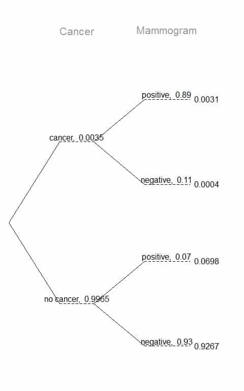
We can plot the data as a tree diagram with primary branches for cancer or no cancer presence with marginal probabilities 0.0035 and 0.9965 respectively.
The secondary branches are conditioned on the cancer presence.
From the information provided, the probability that the test is negative (mammogram =negative) given that the woman has cancer (cancer = cancer) is 0.11.
So, the probability that the test is positive (mammogram = positive) given that the woman has cancer (cancer = cancer) is 1-0.11 = 0.89.
From the information provided, the probability that the test is positive (mammogram = positive) given that the woman has not cancer (cancer = no cancer) is 0.07.
So, the probability that the test is negative (mammogram = negative) given that the woman has no cancer (cancer = no cancer) is 1-0.07 = 0.93.
We construct joint probabilities at the end of each branch in our tree by multiplying the numbers we come across as we move from left to right.
The mammogram results are conditioned on the cancer presence.
However, if we want to find the inverted conditional probability that the patient has breast cancer when her mammogram result was positive.
From the rule of conditional probability,
p(has cancer|mammogram positive) = p(has cancer and mammogram positive)/p(mammogram positive).
p(has cancer and mammogram positive) = Joint probability at the end of the secondary branch for cancer presence and positive mammogram = 0.0031.
p(mammogram positive) = Joint probability for cancer presence and positive mammogram+ Joint probability for no cancer and positive mammogram = 0.0031+0.0698 = 0.0729.
p(has cancer|mammogram positive) = p(has cancer and mammogram positive)/p(mammogram positive) = 0.0031/0.0729 = 0.0425 or 4.25%.
Thus, even if a patient (from Canadian women) has a positive mammogram screening, there is only a 4.25% chance that she has breast cancer.
4. Bayes theorem formula
The Bayes theorem for two events or outcomes A and B is:
P(A|B)=(P(B|A)XP(A))/(P(B))
Where:
P(A|B) = conditional probability of A given that B event happened.
P(B|A) = conditional probability of B given that A event happened.
P(A) = marginal probability of A event.
P(B) = marginal probability of B event.
In the above example of mammogram results, p(has cancer|mammogram positive) = p(mammogram positive|has cancer) X p(has cancer)/p(mammogram positive) = 0.89 X 0.0035/0.0729 = 0.0427 or 4.27%.
This is the same percentage calculated above, the difference due to rounding error.
5. When to use Bayes theorem?
When we have two events, A and B, if we know the conditional probability (B|A), we can use the Bayes theorem to find out the inverted conditional probability (A|B) without the need to plot the data as a tree diagram.
– Example 1
A study in 1979 surveyed 445 student-parent pairs for Marijuana use.
Reference:
Ellis GJ and Stone LH. 1979. Marijuana Use in College: An Evaluation of a Modeling Explanation. Youth and Society 10:323-334.
The results of this study are shown in the following table.
| not | used | Sum |
not | 0.3169 | 0.1910 | 0.5079 |
uses | 0.2112 | 0.2809 | 0.4921 |
Sum | 0.5281 | 0.4719 | 1.0000 |
The “not” and “used” columns for parents that did not use and used Marijuana respectively.
The “not” and “uses” rows for students that did not use and used Marijuana respectively.
We call these probabilities joint probabilities because they for two variables (student use and parent use).
From the rule of conditional probability, the probability of student use given that his parent use = p(student use|parent use) = p(student use and parent use)/p(parent use) = 0.2809/0.4719 = 0.5953.
Using the same rule, we can calculate the inverted probability which is the probability of parent use given that his son use = p(parent use|student use) = p(student use and parent use)/p(student use) = 0.2809/0.4921 = 0.5708.
Or using the Bayes theorem, p(parent use|student use) = p(student use|parent use) X p(parent use)/p(student use) = 0.5953 X 0.4719/0.4921 = 0.5708.
– Example 2
An Experiment involving acupuncture and sham acupuncture (as placebo) in the treatment of migraines has found the following results.
Reference:
G. Allais et al. Ear acupuncture in the treatment of migraine attacks: a randomized trial on the efficacy of appropriate versus inappropriate acupoints. In: Neurological Sci. 32.1 (2011), pp. 173-175.
| no | yes | Sum |
control | 0.4944 | 0.0225 | 0.5169 |
treatment | 0.3708 | 0.1124 | 0.4831 |
Sum | 0.8652 | 0.1348 | 1.0000 |
The “no” and “yes” columns for participants who were not relieved from pain and relieved from pain respectively.
The “control” and “treatment” rows for control and treatment participants respectively.
We call these probabilities joint probabilities because they for two variables (treatment use and pain relief).
The probability of participant was in the control group given that he had a pain relieve= p(control|pain relieve) = p(pain relieve and control)/p(pain relieve) = 0.0225/0.1348 = 0.1669.
The inverted probability which is the probability of pain relieve given that participant was in the control group = p(pain relieve|control) = p(pain relieve and control)/p(control) = 0.0225/0.5169 = 0.0435.
Or using the Bayes theorem,
p(pain relieve|control) = p(control|pain relieve) X p(pain relieve)/p(control) = 0.1669 X 0.1348/0.5169 = 0.0435.
6. Practice questions
1. Researchers were interested in the relationship between learning status (average learner (‘AL’) and slow learner (‘SL’)) and the gender of children (female (“F”) and male (“M”)).
The data from 146 randomly sampled students in rural New South Wales, Australia, in a particular school year showed the following results.
Source:
Venables WN, Ripley BD. 2002. Modern Applied Statistics with S. Fourth Edition. New York: Springer.
| AL | SL | Sum |
F | 0.2740 | 0.2740 | 0.5479 |
M | 0.2945 | 0.1575 | 0.4521 |
Sum | 0.5685 | 0.4315 | 1.0000 |
The probability of student was a female given that she was a slow learner (“SL”)= p(F|SL) = p(F and SL)/p(SL) = 0.2740/0.4315 = 0.635.
Calculate the inverted probability which is the probability of the student was a slow learner given that she was a female (p(SL|F))?
2. In the previous study, researchers were interested in the relationship between learning status (average learner (‘AL’) and slow learner (‘SL’)) and the children’s ethnicity (Aboriginal (“A”) or not (“N”)).
The data from 146 randomly sampled students in rural New South Wales, Australia, in a particular school year showed the following results.
| AL | SL | Sum |
A | 0.2740 | 0.1986 | 0.4726 |
N | 0.2945 | 0.2329 | 0.5274 |
Sum | 0.5685 | 0.4315 | 1.0000 |
The probability of student was an Aboriginal given that he was a slow learner (“SL”)= p(A|SL) = p(A and SL)/p(SL) = 0.1986/0.4315 = 0.4603.
Calculate the inverted probability which is the probability of the student was a slow learner given that he was an Aboriginal (p(SL|A))?
3. Three treatments were compared to test their relative efficacy (effectiveness) in treating Type 2 Diabetes in patients aged 10-17.
Each of the 699 patients in the experiment was randomized to one of the following treatments:
- continued treatment with metformin (coded as met),
- formin combined with rosiglitazone (coded as rosi), or
- a lifestyle-intervention program (coded as lifestyle).
The primary outcome was a lack of glycemic control (or not).
Lacking glycemic control means the patient still needed insulin and failure of the treatment.
Source:
Zeitler P, et al. 2012. A Clinical Trial to Maintain Glycemic Control in Youth with Type 2 Diabetes. N Engl J Med.
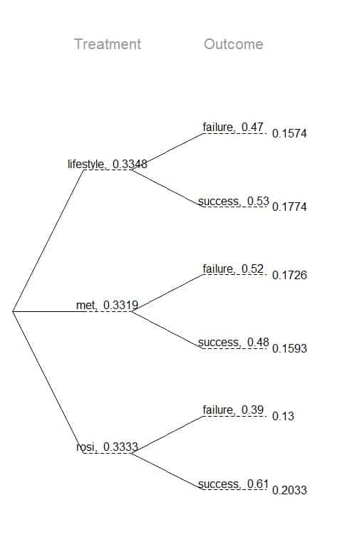 From this tree diagram, find these conditional probabilities:
p(failure|lifestyle).
p(success|rosi).
4. From the previous example, find the inverted probabilities:
p(lifestyle|failure).
p(rosi|success).
5. A poll about the use of full-body airport scanners has shown the following results.
Source:
S. Condon. Poll: 4 in 5 Support Full-Body Airport Scanners. In: CBS News (2010).
| Democrat | Independent | Republican | Sum |
do not know / no answer | 15 | 22 | 16 | 53 |
should | 299 | 351 | 264 | 914 |
should not | 55 | 77 | 38 | 170 |
Sum | 369 | 450 | 318 | 1137 |
Calculate:
The joint probability of being “Democrat” and answer with “should”.
The marginal probability of being “Democrat”.
The conditional probability of answering “should” given that the person is “Democrat”.
7. Answer key
1. p(SL|F) = p(SL and F)/p(F) = 0.2740/0.5479 = 0.5000.
Or using the Bayes theorem,
p(SL|F) = p(F|SL) X p(SL)/p(F) = 0.635 X 0.4315/0.5479 = 0.5000.
2. p(SL|A) = p(SL and A)/p(A) = 0.1986/0.4726 = 0.4202.
Or using the Bayes theorem,
p(SL|A) = p(A|SL) X p(SL)/p(A) = 0.4603 X 0.4315/0.4726 = 0.4203.
3. From the tree diagram,
p(failure|lifestyle) = probability of failure given that the patient was in the lifestyle group = 0.47 or 47%.
p(success|rosi) = probability of success given that the patient was in the rosi group = 0.61 or 61%.
4. Using the Bayes theorem formula:
P(A|B)=(P(B|A)XP(A))/(P(B))
p(lifestyle|failure) = p(failure|lifestyle) X p(lifestyle)/p(failure).
we have:
p(failure|lifestyle) = 0.47.
p(lifestyle) = 0.3348.
p(failure) = sum of joint probabilities = p(lifestyle and failure)+ p(met and failure) + p(rosi and failure) = 0.1574+0.1726+0.13 = 0.46.
So:
p(lifestyle|failure) = p(failure|lifestyle) X p(lifestyle)/p(failure) = 0.47 X 0.3348/0.46 = 0.342 or 34.2%.
For the second probability:
p(rosi|success) = p(success|rosi) X p(rosi)/p(success).
we have:
p(success|rosi) = 0.61.
p(rosi) = 0.3333.
p(success) = sum of joint probabilities = p(lifestyle and success)+ p(met and success) + p(rosi and success) = 0.1774+0.1593+0.2033 = 0.54.
So:
p(rosi|success) = p(success|rosi) X p(rosi)/p(success) = 0.61 X 0.3333/0.54 = 0.3765 or 37.65%.
5. The joint probability of being “Democrat” and answer with “should” = the number of “Democrat” and responded with “should”/total data = 299/1137 = 0.263 or 26.3%.
The marginal probability of being “Democrat” = sum of “Democrat”/total data = 369/1137 = 0.325 or 32.5%.
The conditional probability of answering “should” given that the person is “Democrat” = p(should|Democrat) = p(should and Democrat)/p(Democrat) = 0.263/0.325 = 299/369 = 0.81 or 81%.