JUMP TO TOPIC
Bernoulli Distribution – Explanation & Examples
 The definition of the Bernoulli distribution is:
“The Bernoulli distribution is a discrete probability distribution that describes the probability of a random variable with only two outcomes.”
In this topic, we will discuss the Bernoulli distribution from the following aspects:
- What is a Bernoulli distribution?
- When to use Bernoulli distribution?
- Bernoulli distribution formula.
- Practice questions.
- Answer key.
1. What is a Bernoulli distribution?
The Bernoulli distribution is a discrete probability distribution that describes the probability of a random variable with only two outcomes.
In the random process called a Bernoulli trial, the random variable can take one outcome, called a success, with a probability p, or take another outcome, called failure, with a probability q = 1-p.
The success outcome is denoted as 1 and the failure outcome is denoted as 0.
The Bernoulli distribution is a special case of the binomial distribution where a single trial is conducted and the binomial distribution is the sum of repeated Bernoulli trials.
The Bernoulli distribution was named after the Swiss mathematician Jacob Bernoulli.
– Example 1
Tossing a coin can result in only two possible outcomes (head or tail). We call one of these outcomes (head) a success and the other (tail), a failure.
The probability of success (p) or head is 0.5 for a fair coin. The probability of failure (q) or tail = 1-p = 1-0.5 = 0.5.
If we denote head as 1 and tail as 0, we can plot this Bernoulli distribution as follows:
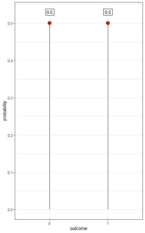 We have two outcomes:
- Tail or 0 with a probability of 0.5.
- Head or 1 with a probability of 0.5 also.
This is an example of a probability mass function where we have the probability for each outcome.
– Example 2
We have an unfair coin where the probability of success (p) or head is 0.8 and the probability of failure (q) or tail = 1-p = 1-0.8 = 0.2.
If we denote head as 1 and tail as 0, we can plot this Bernoulli distribution as follows:

We have two outcomes:
- Tail or 0 with a probability of 0.2.
- Head or 1 with a probability of 0.8.
– Example 3
The prevalence of a certain disease in the general population is 10%.
If we randomly select a person from this population, we can have only two possible outcomes (diseased or healthy person). We call one of these outcomes (diseased person) success and the other (healthy person), a failure.
The probability of success (p) or diseased person is 10% or 0.1. So, the probability of failure (q) or healthy person = 1-p = 1-0.1 = 0.9.
If we denote diseased person as 1 and healthy person as 0, we can plot this Bernoulli distribution as follows:
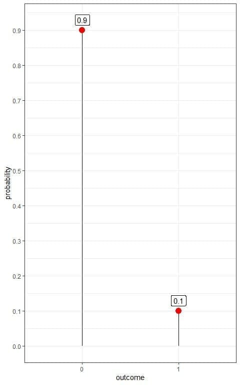
We have two outcomes:
- A healthy person or 0 with a probability of 0.9.
- A diseased person or 1 with a probability of 0.1.
– Example 4
In the above example of disease prevalence of 10%, if We are interested in healthy persons and call the healthy person a success and the diseased person, a failure.
The probability of success (p) or healthy person is 90% or 0.9. So, the probability of failure (q) or diseased person = 1-p = 1-0.9 = 0.1.
If we denote a healthy person as 1 and diseased person as 0, we can plot this Bernoulli distribution as follows:
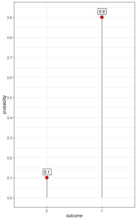
We have two outcomes:
- A healthy person or 1 with a probability of 0.9.
- A diseased person or 0 with a probability of 0.1.
2. When to use Bernoulli distribution?
For a random variable to be described by the Bernoulli distribution:
- The random variable can take only one of two possible outcomes. We call one of these outcomes a success and the other, a failure.
- The probability of success, denoted by p, is the same in every Bernoulli trial.
- The trials are independent, meaning that the outcome in one trial does not affect the outcome in other trials.
We can determine the Bernoulli distribution from the results of different Bernoulli trials.
– Example 1
You are tossing a coin. The random variable equals to 1 if you get a head and 0 if you get a tail.
You tossed the coin 100 times and get the following results:
0 1 0 1 1 0 1 1 1 0 1 0 1 1 0 1 0 0 0 1 1 1 1 1 1 1 1 1 0 0 1 1 1 1 0 0 1 0 0 0 0 0 0 0 0 0 0 0 0 1 0 0 1 0 1 0 0 1 1 0 1 0 0 0 1 0 1 1 1 0 1 1 1 0 0 0 0 1 0 0 0 1 0 1 0 0 1 1 1 0 0 1 0 1 0 0 1 0 0 1.
What is the Bernoulli distribution for this coin?
You can use that data to estimate the probability mass function (or the probability distribution) for tossing this coin.
1. We construct a frequency table for each outcome.
Outcome | frequency |
0 | 53 |
1 | 47 |
2. Add another column for the probability of each outcome.
Probability = frequency/total number of data = frequency/100.
Outcome | frequency | probability |
0 | 53 | 0.53 |
1 | 47 | 0.47 |
The probabilities are >= 0 and sum to 1.
This is a likely fair coin where the probability of heads nearly equals the probability of tails = 0.5.
We do not get exactly 50 heads and 50 tails due to randomness in the process but we get a good approximation to the probability of the fair coin = 0.5.
3. Use the table to plot the Bernoulli distribution for that coin:
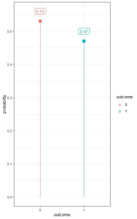
We have two outcomes:
- Head or 1 with a probability of 0.47.
- Tail or 0 with a probability of 0.53.
– Example 2
You screened 50 individuals from a certain population for the presence of hypertension and get the following results:
ID | condition |
1 | normotensive |
2 | normotensive |
3 | normotensive |
4 | normotensive |
5 | normotensive |
6 | normotensive |
7 | normotensive |
8 | normotensive |
9 | normotensive |
10 | normotensive |
11 | hypertensive |
12 | normotensive |
13 | normotensive |
14 | normotensive |
15 | normotensive |
16 | normotensive |
17 | normotensive |
18 | normotensive |
19 | normotensive |
20 | hypertensive |
21 | normotensive |
22 | normotensive |
23 | normotensive |
24 | hypertensive |
25 | normotensive |
26 | normotensive |
27 | normotensive |
28 | normotensive |
29 | normotensive |
30 | normotensive |
31 | hypertensive |
32 | normotensive |
33 | normotensive |
34 | normotensive |
35 | normotensive |
36 | normotensive |
37 | normotensive |
38 | normotensive |
39 | normotensive |
40 | normotensive |
41 | normotensive |
42 | normotensive |
43 | normotensive |
44 | normotensive |
45 | normotensive |
46 | normotensive |
47 | normotensive |
48 | normotensive |
49 | normotensive |
50 | normotensive |
What is the estimated Bernoulli distribution for hypertension in this population?
1. We construct a frequency table for each outcome.
Outcome | frequency |
hypertensive | 4 |
normotensive | 46 |
2. Add another column for the probability of each outcome. As we are interested in hypertension, so we denote hypertensive persons as 1 and normotensive persons as 0.
Probability = frequency/total number of data = frequency/50.
outcome | frequency | probability |
1 | 4 | 0.08 |
0 | 46 | 0.92 |
The probabilities are >= 0 and sum to 1.
3. Use the table to plot the Bernoulli distribution for hypertension:
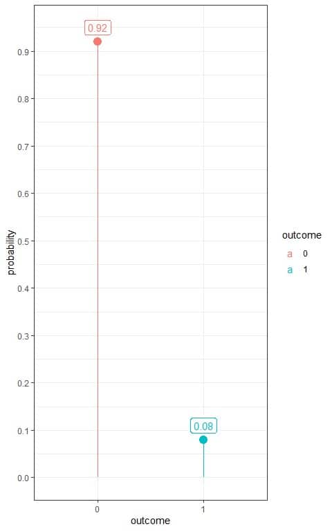
We have two outcomes:
- A hypertensive person or 1 with a probability of 0.08.
- A normotensive person or 0 with a probability of 0.92.
– Example 3
You screened a 100 tablet-sample from two tablet producing machines in a certain factory. We denote 1 for rejected tablets and 0 for accepted tablets and get the following results:
Tablet | machine1 | machine2 |
1 | 0 | 0 |
2 | 0 | 0 |
3 | 0 | 0 |
4 | 0 | 1 |
5 | 0 | 0 |
6 | 0 | 0 |
7 | 0 | 1 |
8 | 0 | 0 |
9 | 0 | 0 |
10 | 0 | 0 |
11 | 1 | 1 |
12 | 0 | 0 |
13 | 0 | 0 |
14 | 0 | 1 |
15 | 0 | 0 |
16 | 0 | 0 |
17 | 0 | 0 |
18 | 0 | 1 |
19 | 0 | 0 |
20 | 1 | 0 |
21 | 0 | 0 |
22 | 0 | 0 |
23 | 0 | 0 |
24 | 1 | 0 |
25 | 0 | 0 |
26 | 0 | 1 |
27 | 0 | 0 |
28 | 0 | 0 |
29 | 0 | 0 |
30 | 0 | 0 |
31 | 1 | 0 |
32 | 0 | 0 |
33 | 0 | 0 |
34 | 0 | 0 |
35 | 0 | 0 |
36 | 0 | 0 |
37 | 0 | 0 |
38 | 0 | 0 |
39 | 0 | 1 |
40 | 0 | 0 |
41 | 0 | 0 |
42 | 0 | 0 |
43 | 0 | 0 |
44 | 0 | 0 |
45 | 0 | 0 |
46 | 0 | 0 |
47 | 0 | 0 |
48 | 0 | 0 |
49 | 0 | 0 |
50 | 0 | 0 |
51 | 0 | 0 |
52 | 0 | 0 |
53 | 0 | 0 |
54 | 0 | 0 |
55 | 0 | 0 |
56 | 0 | 0 |
57 | 0 | 0 |
58 | 0 | 0 |
59 | 0 | 0 |
60 | 0 | 0 |
61 | 0 | 0 |
62 | 0 | 0 |
63 | 0 | 0 |
64 | 0 | 0 |
65 | 0 | 0 |
66 | 0 | 0 |
67 | 0 | 0 |
68 | 0 | 0 |
69 | 0 | 0 |
70 | 0 | 0 |
71 | 0 | 0 |
72 | 0 | 0 |
73 | 0 | 0 |
74 | 0 | 0 |
75 | 0 | 0 |
76 | 0 | 0 |
77 | 0 | 0 |
78 | 0 | 0 |
79 | 0 | 0 |
80 | 0 | 0 |
81 | 0 | 0 |
82 | 0 | 0 |
83 | 0 | 0 |
84 | 0 | 0 |
85 | 0 | 0 |
86 | 0 | 0 |
87 | 1 | 0 |
88 | 0 | 0 |
89 | 0 | 1 |
90 | 0 | 1 |
91 | 0 | 0 |
92 | 0 | 0 |
93 | 0 | 1 |
94 | 0 | 0 |
95 | 0 | 1 |
96 | 0 | 0 |
97 | 0 | 0 |
98 | 0 | 0 |
99 | 0 | 0 |
100 | 0 | 0 |
What is the estimated Bernoulli distribution for rejections from each machine?
1. We construct a frequency table for each outcome.
Outcome | frequency_machine1 | frequency_machine2 |
0 | 95 | 89 |
1 | 5 | 11 |
2. Add another column for the probability of each outcome.
Probability = frequency/total number of data = frequency/100.
Outcome | frequency_machine1 | frequency_machine2 | probability_machine1 | probability_machine2 |
0 | 95 | 89 | 0.95 | 0.89 |
1 | 5 | 11 | 0.05 | 0.11 |
We see that the probability of rejected tablets from the second machine is 0.11 or 11% which is about double the probability from the first machine (0.05 or 5%).
3. Use the table to plot the Bernoulli distribution for these machines:
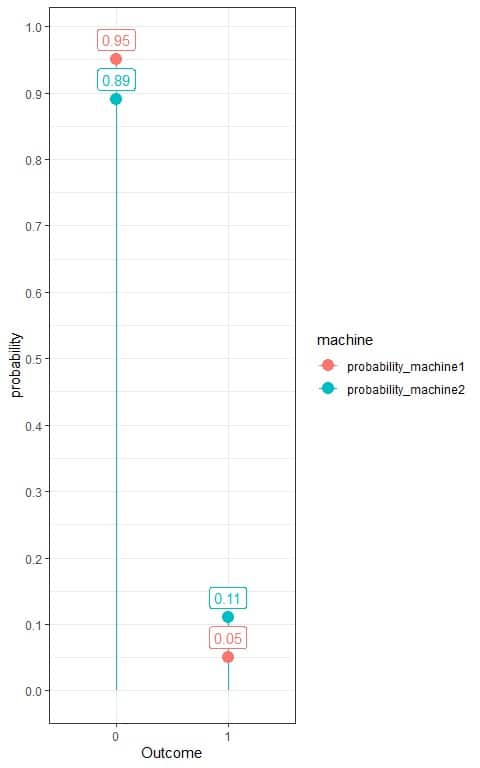
We see that the probability of rejections (outcome = 1) from the first machine is 0.05 or 5%, while the probability of rejections from the second machine is 0.11 or 11%.
4. Bernoulli distribution formula
If the random variable X takes only two outcomes, 0 or 1. The success outcome is denoted as 1 and the failure outcome is denoted as 0, and probability of success p, the probability of any outcome k is given by:
f(k,p)=p^k (1-p)^(1-k)
where:
f(k,p) is the probability of k outcome with a probability of success,p.
p is the probability of success and 1-p is the probability of failure.
This probability mass function can take only two values as we have two outcomes only:
When k =0, f(k,p)=p^k (1-p)^(1-k)=p^0 (1-p)^1 = 1-p.
When k =1, f(k,p)=p^k (1-p)^(1-k)=p^1 (1-p)^0 = p.
So this probability mass function can be rewritten as:
f(k,p)={■(p&”if ” k=1@1-p&”if ” k=0)┤
5. Practice questions
1. The following plot shows the Bernoulli distribution of diabetes in a certain population, where we denote the diabetic person as 1 and healthy person as 0:
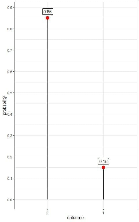
What is the prevalence of diabetes in this population?
2. The following plot shows the Bernoulli distribution of survival from a certain pandemic in some population, where we denote the survived person as 1 and died person as 0:
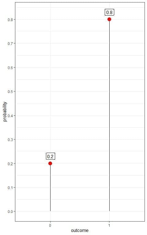
If we know that this population is about 1 million persons. How many persons have survived this pandemic?
3. The following plot shows the Bernoulli distribution of survival from a certain pandemic in 2 populations, population1 and population2, where we denote the survived person as 1 and died person as 0:
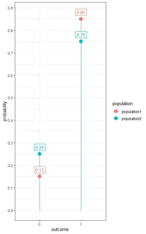
Which population was more susceptible to this pandemic?
4. The following frequency table shows the number of hypertensive patients in a sample of 100 persons randomly selected from a certain population.
We denote hypertensive persons as 1 and normotensive persons as 0.
outcome | frequency |
0 | 94 |
1 | 6 |
What is the estimated Bernoulli distribution for hypertension in this population?
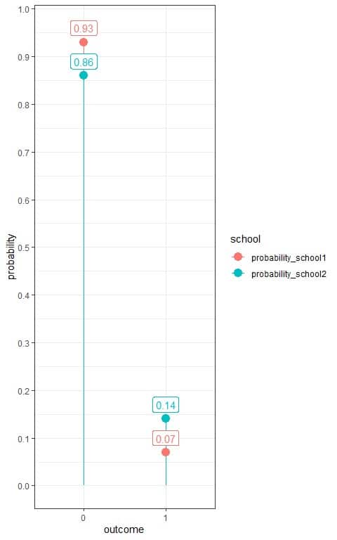
5. The following frequency table shows the number of failed students in a certain exam from 2 schools, school1 and school2.
We are interested in failed students, so we denote failed students as 1 and succeeded students as 0.
outcome | school1 | school2 |
0 | 65 | 86 |
1 | 5 | 14 |
What is the estimated Bernoulli distribution for failure in the 2 schools?
6. Answer key
1. We have two outcomes:
- A healthy person or 0 with a probability of 0.85.
- A diabetic person or 1 with a probability of 0.15.
The prevalence of diabetes in this population = probability of diabetic person = 0.15 or 15%.
2. We have two outcomes:
- A dead person or 0 with a probability of 0.2.
- A survived person or 1 with a probability of 0.8.
For 1 million persons, the number of survivors = 1,000,000 X 0.8 = 800,000 persons.
3. We have two outcomes:
- A dead person or 0.
- A survived person or 1 with a probability.
We see that population2 has more probability of dying (0.25) than population1 (0.15) so population2 was more susceptible.
4. We add another column for the probability of each outcome.
Probability = frequency/total number of data = frequency/100.
outcome | frequency | probability |
0 | 94 | 0.94 |
1 | 6 | 0.06 |
The probabilities are >= 0 and sum to 1.
Use the table to plot the Bernoulli distribution for hypertension:
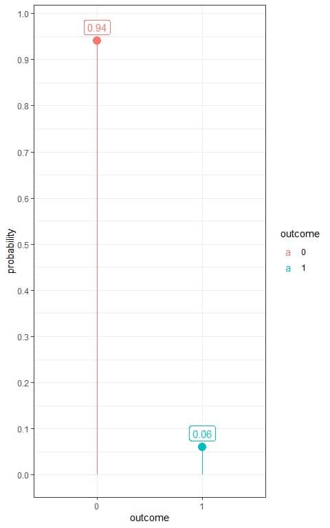
So, this Bernoulli distribution can be written as:
f(k,p)={■(0.06&”if ” [email protected]&”if ” k=0)┤
5. We note that school1 has 70 students, while school2 has 100 students.
Add another column for the probability of each outcome.
For school1, Probability = frequency/total number of data = frequency/70.
For school2, Probability = frequency/total number of data = frequency/100.
outcome | school1 | school2 | probability_school1 | probability_school2 |
0 | 65 | 86 | 0.93 | 0.86 |
1 | 5 | 14 | 0.07 | 0.14 |
We see that the probability of failure for students from school1 is 0.07 or 7% which is half the probability from school2 (0.14 or 14%).
Use the table to plot the Bernoulli distribution for the 2 schools:
For school1, the Bernoulli distribution can be written as:
f(k,p)={■(0.07&”if ” [email protected]&”if ” k=0)┤
and for school2, the Bernoulli distribution can be written as:
f(k,p)={■(0.14&”if ” [email protected]&”if ” k=0)┤