Central Limit Theorem – Explanation & Examples

The definition of the Central Limit Theorem (CLT) is:

“The Central Limit Theorem states that the sampling distribution of a sample statistic is nearly normal and will have on average the true population parameter that is being estimated.”

In this topic, we will discuss the central limit theorem from the following aspects:

1. What is the central limit theorem?
2. When to use the central limit theorem?
3. Central limit theorem conditions for mean.
4. Central limit theorem formula for mean.
5. How to use the central limit theorem formula for mean?
6. Central limit theorem conditions for proportion.
7. Central limit theorem formula for proportion.
8. How to use the central limit theorem for proportion?
9. Practice questions.
10. Answer key.

1. What is the central limit theorem?

The central limit theorem states that the sampling distribution of a sample statistic (like the sample mean or proportion) is nearly normal or bell-shaped and will have on average the true population parameter that is being estimated.

The sampling distribution is a theoretical distribution, that we cannot observe, that describes all the possible values of a sample statistic from random samples of the same size that are taken from the same population.

In real-life research, only one sample is taken with a certain size from a specific population.

There are many types of sample statistics that the CLT can be applied to:

• The sample mean for continuous variables.
• Sample proportion for categorical variables.
• The sample mean difference for comparing 2 continuous variables.
• Sample proportion difference for comparing 2 categorical variables.

We will focus on the application of CLT to sample means and proportions.

Any sample we get randomly from a population is one of many possible samples that we may get by chance.

The sample means or proportions based on certain size vary across different hypothetical samples of the same size.

This variability in sample means or proportions is called the standard error (SE) and is different from the variability of individual values in any single sample, which is called the standard deviation (s).

– Example of the sampling distribution for sample means

We have population data for individual heights. We know that the population mean for these heights is 162.9 cm.

The distribution of heights in this population is normal or bell-shaped as we see from the histogram below.

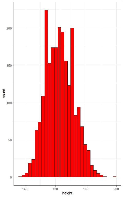
The x-axis is the individual heights and the histogram has a normally distributed shape that is centered around the population mean (plotted as a vertical black line).

Using a computer program, we will take 1000 random samples from this population data, each of size 30 or 100, calculate the sample mean for each sample, and plot the samples’ means as histograms to see their sampling distribution.

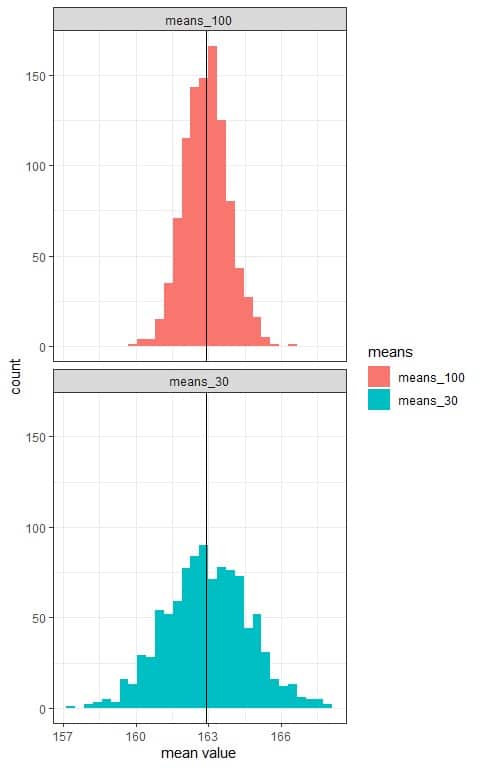
We see that:

• The x-axis is the mean value from each sample.
• We have two histograms, one for the sample means based on 30 sample size (means_30) and the other for the sample means based on 100 sample size (means_100).
• The (sampling) distribution of sample means is normally distributed for both sample sizes (30 and 100).
• The distribution of sample means is centered around the population mean which is plotted as a black vertical line.
• The variability of the sampling distribution decreases with increasing the sample size. The histogram range for means_30 is from 158 cm to 167 cm, while the histogram range for means_100 is from 160 cm to 166 cm.

The CLT also holds when the distribution of the individual observations is not normal as we will see in the following example.

– Example of the sampling distribution for sample means from skewed data

We have population data for individual incomes. We know that the population mean for these incomes is $23599.98.

The distribution of incomes in this population is right-skewed as we see from the histogram below.

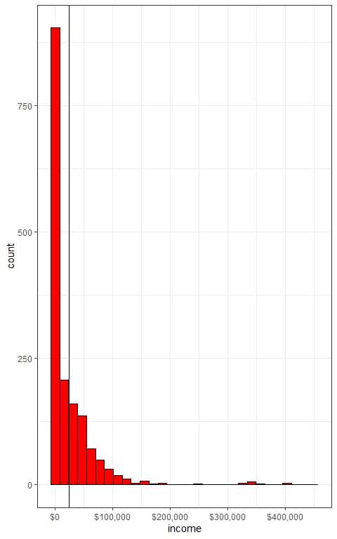
The x-axis is the individual incomes and the histogram has a right-skewed distribution and not centered around the population mean which is plotted as a vertical black line.

Using a computer program, we will take 1000 random samples from this population data, each of size 30 or 100, calculate the sample mean for each sample, and plot the samples’ means as histograms to see their sampling distribution.

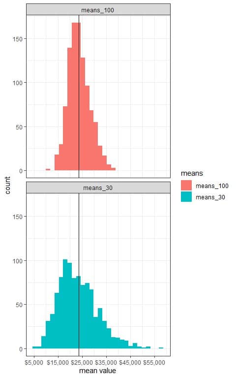
We see that:

• The x-axis is the mean value from each sample.
• We have two histograms, one for the sample means based on 30 sample size (means_30) and the other for the sample means based on 100 sample size (means_100).
• The (sampling) distribution of sample means is normally distributed for both sample sizes (30 and 100).
• The distribution of sample means is nearly symmetric around the population mean which is plotted as a black vertical line.
• The variability of the sampling distribution decreases with increasing the sample size. The histogram range for means_30 is from $5,000 to $50,000, while the histogram range for means_100 is from $10,000 to $40,000.

– Example of the sampling distribution for sample proportions

We have population data for individual smoking habits. We know that the true population proportion for smoking is 0.395 or 39.5%.

We can see the percentage of smoking and non-smoking individuals from the following bar plot.

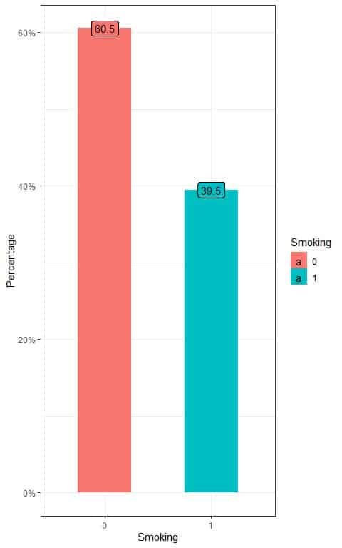
We see that the percentage of non-smoking individuals (smoking = 0) is 60.5% and the percentage of smoking individuals (smoking = 1) is 39.5%.

Using a computer program, we will take 1000 random samples from this population data, each of size 30 or 100, calculate the smoking proportion from each sample, and plot the different sample proportions as histograms to see their sampling distribution.

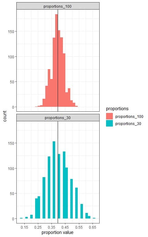
We see that:

• The x-axis is the proportion value from each sample.
• We have two histograms, one for the sample proportions based on 30 sample size (proportions_30) and the other for the sample proportions based on 100 sample size (proportions_100).
• The (sampling) distribution of sample proportions is normally distributed for both sample sizes (30 and 100).
• The distribution of sample proportions is centered around the true population proportion (0.395) which is plotted as a black vertical line.
• The variability of the sampling distribution decreases with increasing the sample size. The histogram range for proportions_30 is from 0.15 to 0.65 (15% to 65%), while the histogram range for proportions_100 is from 0.25 to 0.55 (25% to 55%).

The reason for the decrease in the variability of the distribution with increasing the sample size is that the sample estimates (means or proportions) will be less affected by sample data (individual observations) with increasing the sample size.

2. When to use the central limit theorem?

Two main conditions must be met to apply the central limit theorem:

1. The sample data must be independent of each other.

For example, if the data are randomly sampled from a population, then they are independent.

2. The sample size must be sufficiently large.

We will discuss these in more detail in the following sections.

– Central limit theorem conditions for sample means

1. The sample data must be independent.
2. The sample size must be sufficiently large.

The sample size (n) is at least 30 to apply the CLT to sample means and the sampling distribution of the sample mean will be nearly normal, even if the underlying population distribution of individual observations is not normally distributed.

– Central limit theorem formula for mean

For a large sample of n ≥ 30 independent observations, the sampling distribution of the sample mean ¯x will be nearly normal with:

μ_¯x=μ

and

SE=σ/√n

Where:

μ_¯x is the mean of the sample means with the same size (n).

μ is the population mean.

SE is the standard error or the variability in the sample means.

σ is the population standard deviation. It can be replaced by the sample standard deviation (s) when the sample size is ≥ 30.

3. How to use the central limit theorem for the sample mean?

For any normal distribution, 95% of the data are within 2 (or more accurately 1.96) standard deviations from the mean.

Using the sample mean ¯x as an estimate of the population mean μ and the SE, we can construct a 95% confidence interval that most likely contains the population mean.

95% confidence interval = ¯x±1.96XSE = ¯x±1.96X s/√n

– Interpretation of confidence intervals

A confidence interval gives us a range of possible values for the unknown population parameter (mean or proportion) from which the sample was taken.

The 95% confidence level means that the true population parameter is not necessarily within this interval but for 95% of samples taken from this population and with the same size, the confidence interval generated from them will contain the true population parameter.

In research, when taking a sample and constructing a 95% confidence interval, I do not know if I take one of the good 95% samples that yields interval containing the population value or one of the bad 5% samples that yields interval not containing the population value.

As long as the 95% confidence interval works 95% of the time, we can assume that the constructed interval contains the population value.

– Plotting the confidence intervals of means from different random samples

We have population data for individual heights. We know that the population mean for these heights is 162.9 cm.

Using a computer program, we will take 100 random samples from this population, each of size 100, and calculate the mean, standard deviation, and 95% confidence interval from each sample.

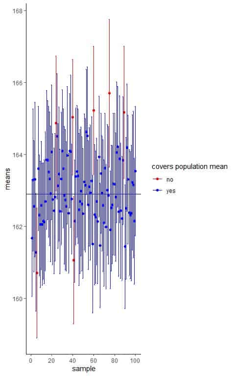
The horizontal black line represents the true population mean (162.9 cm).

The blue or red dots represent the mean height calculated from each random sample.

The error bars represent the 95% confidence interval calculated from each random sample.

We see that only 7 samples create a 95% confidence interval that does not cover the population mean and accounting for 7/100 = 0.07 or 7% so it is very unlikely that the created confidence interval does not cover the population mean.

Example

The following is the weight (in kg) of 30 individuals randomly sampled from a certain population.

What is the 95% confidence interval for the mean weight of this population?

1. Check the Central limit theorem conditions for sample means:

• The sample data must be independent. The data are randomly sampled from the population so they are independent.
• The sample size must be sufficiently large. The sample size = 30 so it is large according to the CLT.

2. Add up all of the weights:

Sum = 2094.2.

3. Count the numbers of items in your data. In this sample, there are 30 items or individuals.

4.l Divide the number you found in step 1 by the number you found in step 2 to get the sample mean.

The sample mean = 2094.2/30 = 69.81 kg.

5. In a table, subtract the mean from each value of your sample.

6. Add another column for the squared differences you found in Step 4.

7. Add up all of the squared differences you found in Step 5.

Sum = 4069.42.

8. Divide the number you get in step 6 by sample size-1 to get the variance. We have 30 numbers so the sample size is 30.

The variance = 4069.42/(30-1) = 140.3248 kg^2.

9. Take the square root of the variance to get the standard deviation.

The standard deviation = √140.3248 = 11.85 kg.

10. Calculate the 95% confidence interval:

95% confidence interval = ¯x±1.96X s/√n = 69.81-1.96X11.85/√30 to 69.81+1.96X11.85/√30 = 65.57 to 74.05 kg.

We are 95% confident that the true population mean weight is between 65.57 and 74.05 kg.

– Central limit theorem conditions for proportion

The sample data must be independent. If the sample data are randomly sampled from the population, so they are independent.

The sample size must be sufficiently large.

The sample size (n) is sufficiently large if np ≥ 10 and n(1-p) ≥ 10. p is the population proportion.

– Central limit theorem formula for proportion

For a large sample of n independent observations and np ≥ 10 and n(1-p) ≥ 10, the sampling distribution of the sample proportion p ̂ will be nearly normal with:

μ_p ̂ =p

and

SE=√((p(1-p))/n)

Where:

μ_p ̂ is the mean of the sample proportions with the same size (n).

p is the population proportion. It can be replaced by the sample proportion (p ̂) for calculating the standard error when np ̂≥10 and n(1-p ̂)≥10.

SE is the standard error or the variability in the sample proportions.

4. How to use the central limit theorem for proportion?

Use the sample proportion p ̂ and the sample size (n) to confirm that np ̂≥10 and n(1-p ̂)≥10.

Use the sample proportion p ̂ and the sample size (n) to construct a 95% confidence interval that most likely contains the population proportion.

95% confidence interval = p ̂±1.96XSE = p ̂±1.96X√((p ̂(1-p ̂))/n).

– Plotting the confidence intervals of proportions from different random samples

We have population data for individual smoking habits. We know that the true population proportion for smoking is 0.395 or 39.5%.

Using a computer program, we will take 100 random samples from this population, each of size 100, and calculate the smoking proportion, standard error, and the 95% confidence interval from each sample.

Note If the sample size is 100 and p = 0.395 (for a perfect sample) so, np = 100X0.395 = 39.5 and n(1-p) = 100X(1-0.395) = 60.5. Both numbers are ≥10.

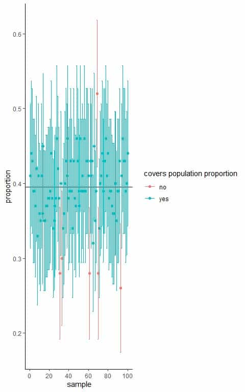
The horizontal black line represents the true population proportion of smoking persons (0.395).

The blue or red dots represent the smoking proportion calculated from each random sample.

The error bars represent the 95% confidence interval calculated from each random sample.

We see that only 6 samples create a 95% confidence interval that does not cover the population proportion and accounting for 6/100 = 0.06 or 6% so it is very unlikely that the created confidence interval does not cover the population proportion.

Example

The following is the smoking habit of 30 individuals randomly sampled from a certain population. When smoke = 1, this means a smoking individual, and when smoke = 0, this means a non-smoking individual.

What is the 95% confidence interval for the smoking proportion in this population

1. Check the Central limit theorem conditions for a sample proportion:

• The sample data must be independent. The data are randomly sampled from the population so they are independent.
• The sample size must be sufficiently large so that np ̂≥10 and n(1-p ̂)≥10.

2. Divide the number of smoking individuals by the sample size to get the sample proportion. We have 12 ones or 12 smoking individuals in our data.

The sample proportion = p ̂ = 12/30 = 0.4.

np ̂ = 30X0.4 = 12 and n(1-p ̂) = 30X0.6 = 18.

Both numbers are greater than 10 so we can use the CLT for sample proportions.

3. Calculate the 95% confidence interval:

95% confidence interval = p ̂±1.96X√((p ̂(1-p ̂))/n) = 0.4-1.96X√(0.4X0.6/30) to 0.4+1.96X√(0.4X0.6/30) = 0.225 to 0.575.

We are 95% confident that the true population proportion for smoking is between 0.225 or 22.5% and 0.575 or 57.5%.

5. Practice questions

1. The following table contains some summary statistics of the daily temperature measurements in degrees Fahrenheit (Temp) randomly sampled from the full daily data.

where n is the sample size and sd is the standard deviation.

What is the 95% confidence interval for the mean Temperature in this data?

2. The following table contains some summary statistics of the hours worked per week (hrs_work) for some persons randomly sampled from a certain population.

where n is the sample size and sd is the standard deviation.

What is the 95% confidence interval for the mean hours worked per week in this population?

3. To overcome the problems of the previous sample, we get a larger random sample and get the following table for some summary statistics of the hours worked per week (hrs_work).

What is the 95% confidence interval for the mean hours worked per week in this population?

4. The following table contains some summary statistics of the length of gestation, in days, from a random sample of pregnant women.

What is the 95% confidence interval for the mean gestational length in the population from which these pregnant women were sampled?

5. The following frequency table shows the gender distribution of a random sample from a certain population.

What is the 95% confidence interval for the female proportion in this population?
What is the 95% confidence interval for the male proportion in this population?

6. Answer key

1. Check the Central limit theorem conditions for a sample mean:

The sample data is independent because they are randomly sampled from the full daily data.

The sample size is large because it is larger than 30.

Calculate the 95% confidence interval:

95% confidence interval = ¯x±1.96X s/√n = 77.9-1.96X9.465/√153 to 77.9+1.96X9.465/√153 = 76.40 to 79.40 degrees Fahrenheit.

We are 95% confident that the full daily data mean temperature is between 76.40 to 79.40 degrees Fahrenheit.

2. Check the Central limit theorem conditions for a sample mean:

The sample data is independent because they are randomly sampled from the population.

The sample size is not large because it is smaller than 30.

We can not calculate the 95% confidence interval from this data.

3. Check the Central limit theorem conditions for a sample mean:

The sample data is independent because they are randomly sampled from the population.

The sample size is large because it is larger than 30.

Calculate the 95% confidence interval:

95% confidence interval = ¯x±1.96X s/√n = 39-1.96X16.307/√42 to 39+1.96X16.307/√42 = 34.1 to 43.9 hours.

We are 95% confident that the population mean for weekly working hours is between 34.1 to 43.9 hours.

4. Check the Central limit theorem conditions for a sample mean:

The sample data is independent because they are randomly sampled from the population.

The sample size is large because it is larger than 30.

Calculate the 95% confidence interval:

95% confidence interval = ¯x±1.96X s/√n = 280.929-1.96X17.225/√98 to 280.929+1.96X17.225/√98 = 277.52 to 284.34 days.

We are 95% confident that the population mean gestational length is between 277.52 to 284.34 days.

5. Check the Central limit theorem conditions for a sample proportion:

The sample data is independent because it is a random sample.

The sample size must be sufficiently large so that np ̂≥10 and n(1-p ̂)≥10.

To get the sample proportion for females, we have 41 females and 59 males with a total = 100.

The sample proportion for females = 41/100 = 0.41.

np ̂ = 100X0.41 = 41 and n(1-p ̂) = 100X0.59 = 59.

Both numbers are greater than 10 so we can use the CLT for the sample proportion of females.

The sample proportion for males = 59/100 = 0.59.

np ̂ = 100X0.59 = 59 and n(1-p ̂) = 100X0.41 = 41.

Both numbers are greater than 10 so we can use the CLT for the sample proportion of males.

Calculate the 95% confidence interval:

95% confidence interval of the female proportion = p ̂±1.96X√((p ̂(1-p ̂))/n) = 0.41-1.96X√(0.41X0.59/100) to 0.41+1.96X√(0.41X0.59/100) = 0.314 to 0.506.

We are 95% confident that the true population proportion for females is between 0.314 to 0.506 or 31.4% to 50.6%.

So, we are 95% confident that the true population proportion for males is between (1-0.314) to (1-0.506) or between 0.686 to 0.494.

Previous Lesson | Main Page | Next Lesson