Change of Variables in Multiple Integrals – Technique, Steps, and Examples
Knowing how to
change variables in multiple integrals allows us to simplify our process of integrating complex functions. There are instances when we need to rewrite the integral of a function in the Cartesian form to its polar form so that we can easily evaluate them. In this discussion, we’ll extend this understanding of how we can apply this knowledge to change variables in multiple integrals as well.
The change of variables in multiple integrals is most helpful when we need to find simpler ways to integrate an expression over a complex region. We can label these changes in multiple integrals as transformations.In the past, we’ve learned how to rewrite single integrals using the u-substitution method. This has helped us integrate complex single variable functions by rewriting them into simpler expressions. We’ve extended this knowledge to double integrals and learned how to rewrite them in their polar forms.Now that we’re working with multiple integrals, it is equally essential that we extend our previous knowledge and learn how to change the variables in multiple integrals for general regions. By the end of this discussion, you’ll understand how planar transformations and Jacobian determinants are essential in the entire process. For now, let’s break down the key concepts we need to understand the process completely.
How To Change Variables in Multiple Integrals?
We can change variables in multiple integrals by applying to utilize
planar transformations – these are functions we use to transform one region to another by changing their variables. As an example, let us show you a visualization of how a region, $H$, in the Cartesian $uv$-plane is transformed to a region, $S$, expressed in the Cartesian $xy$-plane.
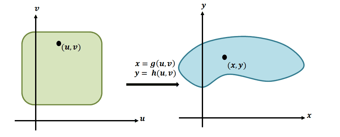
Throughout the discussion, we assume that the partial derivatives are continuous for both regions. Meaning, for our two graphs, the partial derivatives of $g$ and $h$ with respect to both $u$ and $v$ exist and are continuous. We’ll learn more about this process later!For now, let’s take a quick refresher on how we changed variables for single and double integrals. This will help us understand how we’ve established similar rules for multiple integrals. In the past, we’ve learned that we can apply the u-substitution to rewrite the function into a simpler one. This allows us to easily apply the integral properties and formulas as well.\begin{aligned} \int_{1}^{2} x(x^2 – 1)^3 \phantom{x}dx\end{aligned}For this example, we can let $u = g(x)$ represent $x^2 – 1$, so $du = 2x \phantom{x} dx$ or $x \phantom{x}dx = \dfrac{1}{2} \phantom{x}du$. This also means that our limits will have to change by evaluating them at $g(x)$.
| \begin{aligned}\boldsymbol{x = 1 \rightarrow g(1)}\end{aligned} | \begin{aligned}\boldsymbol{x = 2 \rightarrow g(2)}\end{aligned} |
| \begin{aligned}x &= 1\\ g(1) &= 1^2 – 1\\&= 0 \end{aligned} | \begin{aligned}x &= 2\\ g(2) &= 2^2 – 1\\&= 3 \end{aligned} |
With these transformations, we can rewrite and evaluate our integral in terms of $u$ as shown below.\begin{aligned} \int_{1}^{2} x(x^2 – 1)^3 \phantom{x}dx &= \int_{0}^{3} u^3 \cdot \dfrac{1}{2} \phantom{x}du\\&= \dfrac{1}{2}\left[\dfrac{u^4}{4} \right ]_{0}^{3}\\&= \dfrac{1}{8}(3)^4\\&= \dfrac{81}{8}\end{aligned}This reminds us why the u-substitution method is such an important integration technique and will get a long way when you master it. More importantly, this technique is actually our first glimpse on function and limit transformations: we’ve rewritten the function in terms of $x$ to a function in terms of $u$. In fact, we can generalize this rule using the formula shown below.\begin{aligned}\int_{a}^{b} f(x)\phantom{x}dx &= \int_{c = g(a)}^{d = g(b)} f[g(u)] g^{\prime}(u) \phantom{x}du\end{aligned}In fact, we apply a similar process when rewriting double integrals in polar coordinates. This time, we’re working with two variables and functions.\begin{aligned} x &\rightarrow f(r, \theta) = r \cos \theta\\y &\rightarrow g(r, \theta) = r \sin \theta \\dxdy &\rightarrow dA = r drd\theta\end{aligned}These expressions will lead us to the general form of double integrals in polar coordinates as shown below.\begin{aligned}\int \int_{R} f(x, y) \phantom{x}dA &= \int \int_{S} (r \cos \theta, r\sin \theta) \phantom{x}rdrd\theta\end{aligned}
Planar Transformation for Multiple Integrals
Now that we’ve done a quick recap on our substitution techniques in the past, let’s go back to
planar transformations. As we have shown in our earlier examples, it’s possible for us to rewrite functions expression in one variable to another – by accounting for their region’s transformation.

To better understand how planar transformation works, take a look at the transformation shown above. Let’s say we’re working with the planar transformation, $T(r, \theta) = (x = r\cos \theta, y = r\sin \theta)$. The region on the left shows the polar rectangle in the $r\theta$ -plane where any subregion will be contained in the following bounds: $ 0 \leq r \leq 1$ and $0 \leq \theta \leq \dfrac{\pi}{2}$. We can define $T$ in $xy$-plane as a quadrant of a full circle that satisfies the following equations:
\begin{aligned}r^2 = x^2 + y^2\\\tan \theta = \dfrac{y}{x}\end{aligned}
As we have discussed earlier, this planar transformation is important when writing double integrals in polar coordinates. We can extend this idea to account of transformations defined by other functions.
Using Jacobians When Changing Variables in Multiple Integral
The Jacobians of different transformations allow us to generalize the process of changing variables in two or more integrals. We define the Jacobian of a transformation, $T(u, v) = (g(u, v ), h(u, v))$ as shown below.\begin{aligned}J(u, v) &= \left|\dfrac{\partial (x, y)}{\partial (u, v)} \right|\\&=\begin{vmatrix}\dfrac{\partial x}{\partial u} &\dfrac{\partial y}{\partial u} \\ \dfrac{\partial x}{\partial v}& \dfrac{\partial y}{\partial v}\end{vmatrix}\\&= \left(\dfrac{\partial x}{\partial u}\dfrac{\partial y}{\partial v} – \dfrac{\partial x}{\partial v}\dfrac{\partial y}{\partial u} \right ) \end{aligned}Through the Jacobian determinant, we can now rewrite integrals using their partial derivatives for $x$ and $y$. For example, if we have the transformation, $T(u, v) = (2u^2 + 4v^2, 3uv)$, where we define $x$ as the first component and $y$ as the second component. The Jacobian determinant of the transformation is as shown below.
| \begin{aligned}\dfrac{\partial x}{\partial u} &= 4u\\\dfrac{\partial x}{\partial v} &= 8v\\\dfrac{\partial y}{\partial u} &= 3v\\\dfrac{\partial y}{\partial v} &= 3u \end{aligned} | \begin{aligned}J(u, v) &=\begin{vmatrix}\dfrac{\partial x}{\partial u} &\dfrac{\partial y}{\partial u} \\ \dfrac{\partial x}{\partial v}& \dfrac{\partial y}{\partial v}\end{vmatrix}\\&= \begin{vmatrix} 4u & 3v \\ 8v& 3u\end{vmatrix}\\&= [3v(8v) – 4u(3u)]\\&=24v^2 – 12u^2 \end{aligned} |
How does it help us in changing variables?
The Jacobian determinant represents the region that we’re integrating over in our new integral. Meaning, for our transformed double integral, the region, $dA$ is now equal to $(24v^2 – 12u^2) \phantom{x}du dV$.We can extend the definition of Jacobian determinants for three variables: this time, we need to find $J(u, v, w)$.
| \begin{aligned}J(u, v, w) &= \left|\dfrac{\partial (x, y, z)}{\partial (u, v, w)} \right|\\&=\begin{vmatrix}\dfrac{\partial x}{\partial u} &\dfrac{\partial y}{\partial u} &\dfrac{\partial z}{\partial u}\\ \dfrac{\partial x}{\partial v}& \dfrac{\partial y}{\partial v}& \dfrac{\partial z}{\partial v}\\\dfrac{\partial x}{\partial w} &\dfrac{\partial y}{\partial w} & \dfrac{\partial z}{\partial w}&\end{vmatrix}\end{aligned} | \begin{aligned}J(u, v, w) &= \left|\dfrac{\partial (x, y, z)}{\partial (u, v, w)} \right|\\&=\begin{vmatrix}\dfrac{\partial x}{\partial u} &\dfrac{\partial x}{\partial v} &\dfrac{\partial x}{\partial w}\\ \dfrac{\partial y}{\partial u}& \dfrac{\partial y}{\partial v}& \dfrac{\partial y}{\partial w}\\\dfrac{\partial z}{\partial u} &\dfrac{\partial z}{\partial v} & \dfrac{\partial z}{\partial w}&\end{vmatrix}\end{aligned} |
Both Jacobian determinants are equivalent to each other and we can evaluate either to find the value of $J(u, v,w )$. Now, let us establish the rules for changing variables for double and triple integrals using Jacobian determinants.
| CHANGE OF VARIABLES USING JACOBIAN DETERMINANTS |
| $J(u, v)$ | Suppose that $T(u, v) = (x, y)$ represents the transformation and $J(u, v)$ is the nonzero Jacobian for the region, we have the following:\begin{aligned}\int \int_{R} \phantom{x} dA &= \int \int_S f(g(u, v), h(u, v)) J(u, v) \phantom{x} dudv\end{aligned} |
| $J(u, v, w)$ | Suppose that $T(u, v, w) = (x, y, z)$ represents the transformation and $J(u, v)$ is the nonzero Jacobian for the region, we have the following:\begin{aligned}\int \int \int_{R} F(x, y,z) \phantom{x} dV &= \int \int \int_E f(g(u, v, w), h(u, v, w), m(u, v, w)) J(u, v, w) \phantom{x} dudvdw\end{aligned} |
Let’s now break down the
steps we need to change the variables in multiple integrals.
- Sketch the region of the function and identify the equations forming the boundary.
- Establish the appropriate expressions for the transformations: $\{x = g(u, v), y = h(u, v)\}$ or $\{x = g(u, v, w), y = h(u, v, w), z = m(u, v, w)\}$ .
- Set up the limits given the $uv$-plane.
- Use the partial derivatives of $x$, $y$, $z$, or even more variables and write down the Jacobian determinant.
- Rewrite $dA$, normally $dxdy$ or $dxdydz$, as $J(u, v) dudv$ or $J(u,v, w) du dv dw$.
We’ll show you a couple of examples to show you how the process works and work on the remaining problems to further master this topic!
Example 1Evaluate the integral, $\int_{0}^{1} \int_{0}^{\sqrt{4 – x^2}} (x^2 + y^2) \phantom{x} dydx$, by using the change of variables: $x = r \cos \theta$ and $y = r \sin \theta$.
SolutionFirst, sketch the region of integration using the bounds of $y$: lowest bound is $y = 0$ while the highest bound is $y = \sqrt{4 – x^2}$.

First, sketch the region of integration using the bounds of $y$: lowest bound is $y = 0$ while the highest bound is $y = \sqrt{4 – x^2}$. Rewriting the upper bound leads us to $x^2 + y^2 = 4$ – a circle with a radius of $2$ units and centered at the origin.\begin{aligned}x^2 + y^2 &= 4\\ (r \cos\theta)^2 + (r \sin\theta)^2 &= 4\\r^2(\sin^2 \theta + \cos^2 \theta) &= 4\\r^2 &= 4\end{aligned}This confirms that our region of integration is a semicircle bounded by the following limits: $0 \leq r \leq 2$ and $0 \leq \theta \leq \dfrac{\pi}{2}$. Now, let’s work on the Jacobian determinant – taking the partial derivatives of $x = r\cos \theta$ and $y = r\sin \theta$ with respect to $r$ and $\theta$.
| \begin{aligned}\dfrac{\partial x}{\partial r} &= \cos \theta\\\dfrac{\partial x}{\partial \theta} &= -r \sin \theta\\\dfrac{\partial y}{\partial r} &= \sin \theta\\\dfrac{\partial y}{\partial \theta} &=r \cos \theta \end{aligned} | \begin{aligned}J(r, \theta) &=\begin{vmatrix}\dfrac{\partial x}{\partial r} &\dfrac{\partial y}{\partial r} \\ \dfrac{\partial x}{\partial \theta}& \dfrac{\partial y}{\partial \theta}\end{vmatrix}\\&= \begin{vmatrix} \cos\theta & \sin\theta\\-r\sin\theta & r\cos\theta \end{vmatrix}\\&= [r\cos^2 \theta – (-r\sin^2 \theta)]\\&= r\end{aligned} |
Now, use the Jacobian determinant to set up $dA$ in terms of $r$ and $\theta$.\begin{aligned}dA &= J(r, \theta) \phantom{x}drd\theta\\&= r \phantom{x}drd\theta \end{aligned}This confirms what we’ve learned in the past: we use $dA = r \phantom{x}drd\theta$ to convert double integrals in polar coordinates. Now, let’s set up our transformed double integral and evaluate the result.\begin{aligned}\int_{0}^{2} \int_{0}^{\sqrt{4 – x^2}} (x^2 + y^2) \phantom{x}dydx &= \int_{0}^{\pi/2} \int_{0}^{2} r^2 J(r, \theta) \phantom{x}drd\theta\\&= \int_{0}^{\pi/2} \int_{0}^{4} r^2 r\phantom{x}drd\theta\\&= \int_{0}^{\pi/2} \int_{0}^{2} r^3\phantom{x}drd\theta\\&= \int_{0}^{\pi/2} 4 \phantom{x}d\theta\\&= 2\pi\end{aligned}Using the Jacobian determinant and changing the variable of double integrals, we’ve shown that $\int_{0}^{1} \int_{0}^{\sqrt{4 – x^2}} (x^2 + y^2) \phantom{x} dydx$ is equal to $2\pi$.
Example 2Rewrite the triple integral, $\int_{0}^{2} \int_{0}^{4} \int_{y/2}^{y/2 + 2} \left(x + \dfrac{z}{4}\right) \phantom{x} dxdydz$, by using the following transformations:\begin{aligned}u &= \dfrac{x -y}{2} \\v &= \dfrac{y}{2}\\w&= \dfrac{z}{4}\end{aligned}
SolutionHere’s a rough sketch of the transformations occurring between the $uvw$ and $xyz$-planes.

Use the three equations and rewrite them with $x$, $y$, and $z$ as at the left-hand side of the equations: $x =2(u + v)$, $y =2v$, and $z=4w$. This means that $f(x, y, z)$ can be rewritten in terms of $u$, $v$, and $w$:\begin{aligned}f(x, y,z) &= x + \dfrac{z}{4}\\&= 2u + 2v + w \end{aligned}Let’s now find the limits of integration when we transform the region in terms of $u$, $w$, and $z$.
| \begin{aligned}\boldsymbol{x \rightarrow u}\end{aligned} | \begin{aligned}\boldsymbol{y \rightarrow v}\end{aligned} | \begin{aligned}\boldsymbol{z \rightarrow w}\end{aligned} |
| \begin{aligned}x &= \dfrac{y}{2}\\ 2(u + v) &= \dfrac{2v}{2}\\4u + 4v&= 2v\\u&= -\dfrac{v}{2}\end{aligned} | \begin{aligned}y &= 0\\ 2v&= 0\\ v&= 0\end{aligned} | \begin{aligned}z &= 0\\ 4w&= 0\\ w&= 0\end{aligned} |
| \begin{aligned}x &= \dfrac{y}{2} + 2\\ 2(u + v) &= \dfrac{2v}{2} + 2\\4u + 4v&= 2v + 4\\u&= -\dfrac{v}{2} + 2\end{aligned} | \begin{aligned}y &= 4\\ 2v&= 4\\ v&= 2\end{aligned} | \begin{aligned}z &= 2\\ 4w&= 2\\ w&= \dfrac{1}{2}\end{aligned} |
Now that we have the limits of integration, it’s time for us to find the Jacobian determinant for the tripe integral.\begin{aligned}J(u, v, w) &=\begin{vmatrix}\dfrac{\partial x}{\partial u} &\dfrac{\partial x}{\partial v} &\dfrac{\partial x}{\partial w}\\ \dfrac{\partial y}{\partial u}& \dfrac{\partial y}{\partial v}& \dfrac{\partial y}{\partial w}\\\dfrac{\partial z}{\partial u} &\dfrac{\partial z}{\partial v} & \dfrac{\partial z}{\partial w}&\end{vmatrix}\\&= \begin{vmatrix}2 & 2 & 0\\ 0& 2& 0\\0 & 0 & 4&\end{vmatrix} \\&= 16\end{aligned}We can now rewrite the triple integral using our function, new limits of integration, as well as the Jacobian determinant.\begin{aligned}\int_{0}^{2} \int_{0}^{4} \int_{y/2}^{y/2 + 2} \left(x + \dfrac{z}{4}\right) \phantom{x} dxdydz &= \int_{0}^{1/2} \int_{0}^{2} \int_{-v/2}^{-v/2 + 2} \left(2u + 2v + w \right) J(u, v, w) \phantom{x} dudvdw \\&= \int_{0}^{1/2} \int_{0}^{2} \int_{-v/2}^{-v/2 + 2} 16\left(2u + 2v + w \right) \phantom{x} dudvdw \\&= 16\int_{0}^{1/2} \int_{0}^{2} \int_{-v/2}^{-v/2 + 2} \left(2u + 2v + w \right) \phantom{x} dudvdw \end{aligned}This shows that $\int_{0}^{2} \int_{0}^{4} \int_{y/2}^{y/2 + 2} \left(x + \dfrac{z}{4}\right) \phantom{x} dxdydz$ is equivalent to $16\int_{0}^{1/2} \int_{0}^{2} \int_{-v/2}^{-v/2 + 2} \left(2u + 2v + w \right) \phantom{x} dudvdw$ – which is a simpler expression to work with!
Practice Questions
1. Evaluate the integral, $\int_{0}^{4} \int_{0}^{\sqrt{4x – x^2}} \sqrt{x^2 + y^2} \phantom{x} dydx$, by using the change of variables: $x = r \cos \theta$ and $y = r \sin \theta$.
2. Evaluate the triple integral, $\int_{8}^{4} \int_{4}^{0} \int_{z}^{z +3} \left(-4y +5 \right) \phantom{x} dxdydz$, by using the following transformations:
\begin{aligned}u &= -(3z – x)\\v &= 4y\\w&= z\end{aligned}
Answer Key
1.$ \int_{0}^{\pi / 2} \int_{0}^{4\cos \theta} r^2 \phantom{x}dr d\theta = \dfrac{128}{9} \approx 14.22$
2. $\int_{8}^{4} \int_{4}^{0} \int_{z}^{z +3} \left(-4y +5 \right) \phantom{x} dxdydz = -144$
Images/mathematical drawings are created with GeoGebra.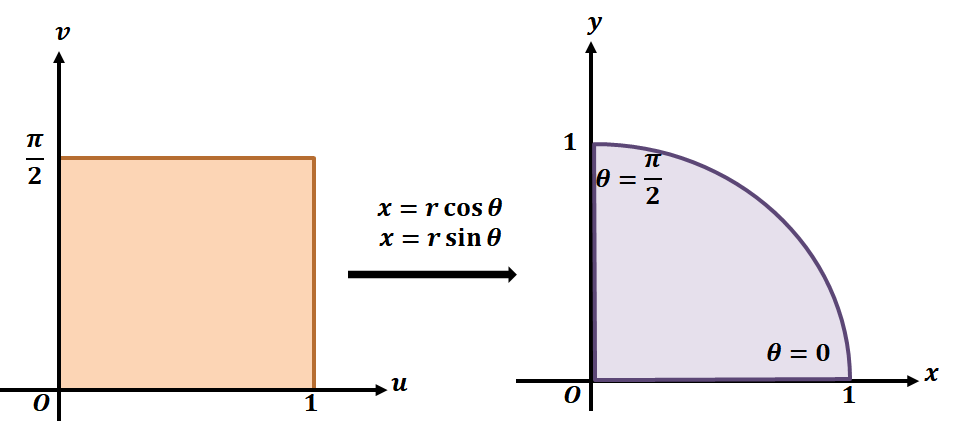 To better understand how planar transformation works, take a look at the transformation shown above. Let’s say we’re working with the planar transformation, $T(r, \theta) = (x = r\cos \theta, y = r\sin \theta)$. The region on the left shows the polar rectangle in the $r\theta$ -plane where any subregion will be contained in the following bounds: $ 0 \leq r \leq 1$ and $0 \leq \theta \leq \dfrac{\pi}{2}$. We can define $T$ in $xy$-plane as a quadrant of a full circle that satisfies the following equations:
\begin{aligned}r^2 = x^2 + y^2\\\tan \theta = \dfrac{y}{x}\end{aligned}
As we have discussed earlier, this planar transformation is important when writing double integrals in polar coordinates. We can extend this idea to account of transformations defined by other functions.
To better understand how planar transformation works, take a look at the transformation shown above. Let’s say we’re working with the planar transformation, $T(r, \theta) = (x = r\cos \theta, y = r\sin \theta)$. The region on the left shows the polar rectangle in the $r\theta$ -plane where any subregion will be contained in the following bounds: $ 0 \leq r \leq 1$ and $0 \leq \theta \leq \dfrac{\pi}{2}$. We can define $T$ in $xy$-plane as a quadrant of a full circle that satisfies the following equations:
\begin{aligned}r^2 = x^2 + y^2\\\tan \theta = \dfrac{y}{x}\end{aligned}
As we have discussed earlier, this planar transformation is important when writing double integrals in polar coordinates. We can extend this idea to account of transformations defined by other functions.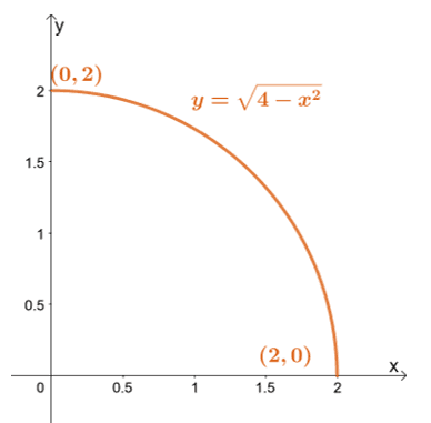 First, sketch the region of integration using the bounds of $y$: lowest bound is $y = 0$ while the highest bound is $y = \sqrt{4 – x^2}$. Rewriting the upper bound leads us to $x^2 + y^2 = 4$ – a circle with a radius of $2$ units and centered at the origin.\begin{aligned}x^2 + y^2 &= 4\\ (r \cos\theta)^2 + (r \sin\theta)^2 &= 4\\r^2(\sin^2 \theta + \cos^2 \theta) &= 4\\r^2 &= 4\end{aligned}This confirms that our region of integration is a semicircle bounded by the following limits: $0 \leq r \leq 2$ and $0 \leq \theta \leq \dfrac{\pi}{2}$. Now, let’s work on the Jacobian determinant – taking the partial derivatives of $x = r\cos \theta$ and $y = r\sin \theta$ with respect to $r$ and $\theta$.
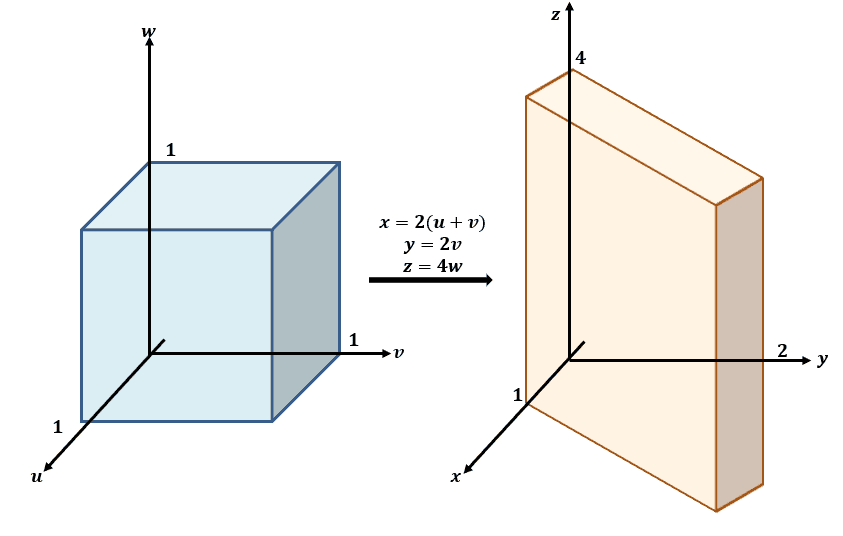 Use the three equations and rewrite them with $x$, $y$, and $z$ as at the left-hand side of the equations: $x =2(u + v)$, $y =2v$, and $z=4w$. This means that $f(x, y, z)$ can be rewritten in terms of $u$, $v$, and $w$:\begin{aligned}f(x, y,z) &= x + \dfrac{z}{4}\\&= 2u + 2v + w \end{aligned}Let’s now find the limits of integration when we transform the region in terms of $u$, $w$, and $z$.