Chebyshev’s Theorem – Explanation & Examples

The definition of Chebyshev’s theorem is:

“The Chebyshev’s theorem is used to find the minimum proportion of data that occur within a certain number of standard deviations from the mean.”

In this topic, we will discuss Chebyshev’s theorem from the following aspects:

1. What is Chebyshev’s theorem?
2. The Chebyshev’s theorem formula.
3. When to use Chebyshev’s theorem?
4. How to use Chebyshev’s theorem?
5. Practice questions.
6. Answer key.

1. What is Chebyshev’s theorem?

Chebyshev’s theorem is used to find the minimum proportion of numerical data that occur within a certain number of standard deviations from the mean.

In normally-distributed numerical data:

• 68% of the data are within 1 standard deviation from the mean.
• 95% of the data are within 2 standard deviations from the mean.
• 99.7% of the data are within 3 standard deviations from the mean.

However, these rules cannot be applied to skewed data or data from other distributions than the normal distribution.

Chebyshev’s theorem is more general and can be applied to a wide range of different distributions.

From Chebyshev’s theorem, we know that:

• At least 75% of the data must lie within 2 standard deviations from the mean.
• At least 88.89% of the data must lie within 3 standard deviations from the mean.

The theorem gives the minimum proportion of the data which must lie within a given number of standard deviations of the mean.

However, the true proportions found within the indicated regions could be greater than what the theorem guarantees.

The theorem is named after the Russian mathematician Pafnuty Chebyshev.

– Example 1

The following are the weights (in kg) of 30 individuals from a certain survey.

54 53 42 49 41 45 69 63 62 72 64 67 81 85 89 79 84 86 101 104 103 108 97 98 126 129 123 119 117 124.

The mean = 84.47 kg and the standard deviation = 27.21 kg.

Validate Chebyshev’s theorem that:

• At least 75% of the data must lie within 2 standard deviations from the mean.
• At least 88.89% of the data must lie within 3 standard deviations from the mean.

We follow these steps:

1. Sort the data and find the minimum and the maximum data values.

The sorted data will be:

41 42 45 49 53 54 62 63 64 67 69 72 79 81 84 85 86 89 97 98 101 103 104 108 117 119 123 124 126 129.

In our data, the minimum value is 41 and the maximum value is 129.

2. Determine the number of bins you need.

The bin boundaries will depend on:

• subtracting the standard deviation multiples from the mean till reaching the minimum value (41).

The mean = 84.47 kg and the standard deviation = 27.21 kg.

84.47-27.21 = 57.26.

84.47-(2X27.21) = 30.05.

• Adding the standard deviation multiples to the mean till reaching the maximum value (129).

84.47+27.21 = 111.68.

84.47+(2X27.21) = 138.89.

The first bin is 30.05-57.26.

The second bin is 57.26-84.47.

The third bin is 84.47-111.68.

The fourth bin is 111.68-138.89.

3. We draw a table of 2 columns. The first column carries the different bins of our data that we created in step 2.

The second column will contain the frequency of weights in each bin.

The bin “30.05-57.26” contains the weights from 30.05 to 57.26, the next bin “57.26-84.47” contains the weights larger than 57.26 till 84.47, and so on.

By looking at the sorted data in step 1, we see that:

• The first 6 numbers (41, 42, 45, 49, 53, 54) are within the first bin “30.05-57.26” so the frequency of this bin is 6.
• The next 9 numbers (62, 63, 64, 67, 69, 72, 79, 81, 84) are within the second bin “57.26-84.47” so the frequency of this bin is 9.
• If you sum these frequencies, you will get 30 which is the total number of data.
  6+9+9+6 = 30.

4. Add a third column for the relative frequency or probability.

Relative frequency = frequency/total data number.

For example, the first bin contains 6 data points or frequency, so the relative frequency = 6/30 = 0.2.

If you sum these relative frequencies, you will get 1.

0.2+0.3+0.3+0.2 = 1.

5. Use the table to plot a relative frequency histogram, where the data bins or ranges on the x-axis and the relative frequency or proportions on the y-axis.

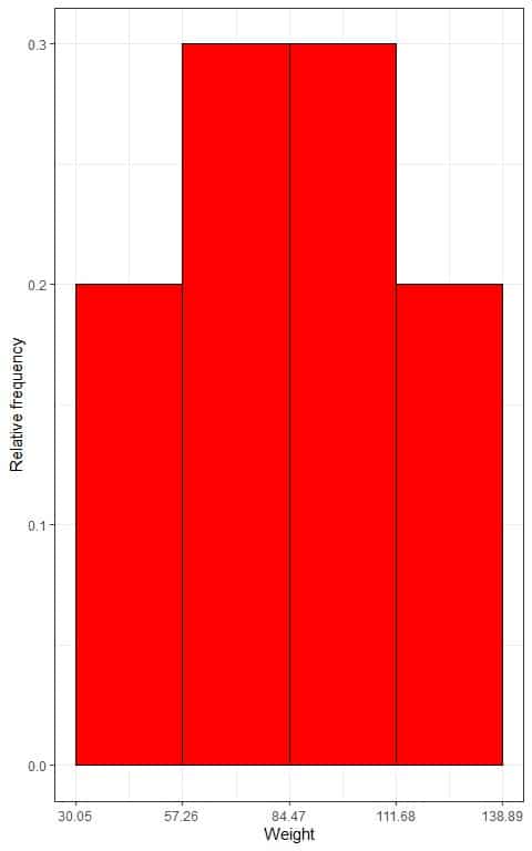
• In relative frequency histograms, the heights or proportions can be interpreted as probabilities. These probabilities can be used to determine the likelihood of certain results occurring within a given interval.
• For example, the relative frequency of the “30.05-57.26” bin is 0.2, so the probability of weights falling in this range is 0.2 or 20%.

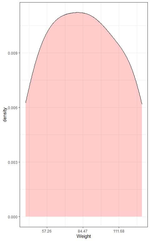
We can also plot a density plot of this data:

6. We can now validate Chebyshev’s theorem that:

• At least 75% of the data must lie within 2 standard deviations from the mean.

The observed proportion for the data within 84.47 +/- (2X27.21) or within 30.05 to 138.89 = sum of relative frequencies within 30.05-138.89 = 1 or 100%.

All our data are within 2 standard deviations from the mean so this statement is true.

• At least 88.89% of the data must lie within 3 standard deviations from the mean.

All our data are within 2 standard deviations from the mean so this statement is true also.

– Example 2

The following are 50 Ozone measurements (in ppb) in New York, May to September 1973.

20 76 16 6 28 85 63 10 24 30 29 23 21 22 18 50 24 11 44 31 71 8 7 21 96 32 73 84 23 45 30 12 13 32 97 21 115 39 39 108 18 28 85 40 135 122 34 11 13 9.

The mean = 41.84 ppb and the standard deviation = 34 ppb.

Validate Chebyshev’s theorem that:

• At least 75% of the data must lie within 2 standard deviations from the mean.
• At least 88.89% of the data must lie within 3 standard deviations from the mean.

We follow these steps:

1. Sort the data and find the minimum and the maximum data values.

The sorted data will be:

6 7 8 9 10 11 11 12 13 13 16 18 18 20 21 21 21 22 23 23 24 24 28 28 29 30 30 31 32 32 34 39 39 40 44 45 50 63 71 73 76 84 85 85 96 97 108 115 122 135.

In our data, the minimum value is 6 and the maximum value is 135.

2. Determine the number of bins you need.

The bin boundaries will depend on:

• subtracting the standard deviation multiples from the mean till reaching the minimum value (6).

The mean = 41.84 ppb and the standard deviation = 34 ppb.

41.84-34 = 7.84.

41.84-(2X34) = -26.16. There are no negative values in our data so it can be rounded to 0.

• Adding the standard deviation multiples to the mean till reaching the maximum value (135).

41.84+34 = 75.84.

41.84+(2X34) = 109.84.

41.84+(3X34) = 143.84.

The first bin is 0-7.84.

The second bin is 7.84-41.84.

The third bin is 41.84-75.84.

The fourth bin is 75.84-109.84.

The fifth bin is 109.84-143.84.

3. We draw a table of 2 columns. The first column carries the different bins of our data that we created in step 2.

The second column will contain the frequency of Ozone measurements in each bin.

The bin “0-7.84” contains the Ozone measurements from 0 to 7.84, the next bin “7.84-41.84” contains the ozone measurements larger than 7.84 to 41.84, and so on.

By looking at the sorted data in step 1, we see that:

• The first 2 numbers (6, 7) are within the first bin “0-7.84” so the frequency of this bin is 2.
• The next 32 numbers (8, 9, 10, 11, 11, 12, 13, 13, 16, 18, 18, 20, 21, 21, 21, 22, 23, 23, 24, 24, 28, 28, 29, 30, 30, 31, 32, 32, 34, 39, 39, 40) are within the second bin “7.84-41.84” so the frequency of this bin is 32.
• If you sum these frequencies, you will get 50 which is the total number of data.

2+32+6+7+3 = 50.

4. Add a third column for the relative frequency or probability.

Relative frequency = frequency/total data number.

For example, the first bin contains 2 data points or frequency, so the relative frequency = 2/50 = 0.04.

If you sum these relative frequencies, you will get 1.

0.04+0.64+0.12+0.14+0.06 = 1.

5. Use the table to plot a relative frequency histogram, where the data bins or ranges on the x-axis and the relative frequency or proportions on the y-axis.

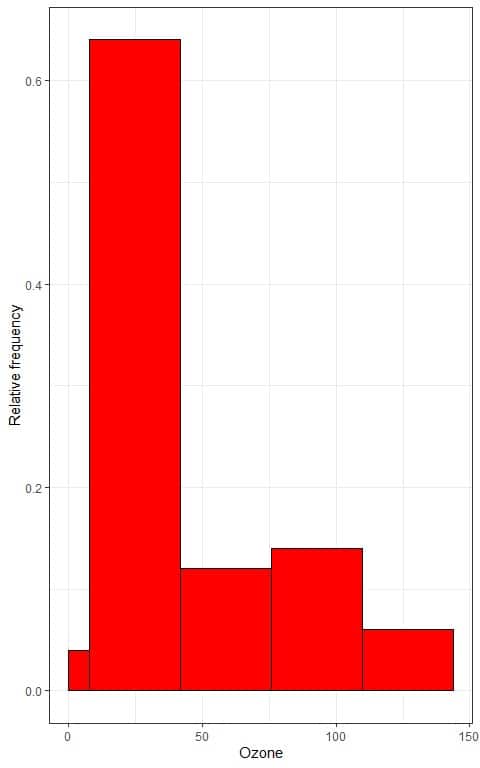
• In relative frequency histograms, the heights or proportions can be interpreted as probabilities. These probabilities can be used to determine the likelihood of certain results occurring within a given interval.
• For example, the relative frequency of the “7.84-41.84” bin is 0.64, so the probability of Ozone falling in this range is 0.64 or 64%.

We can also plot a density plot of this data:

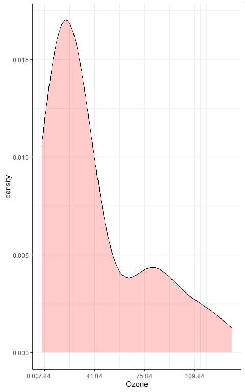
6. We can now validate Chebyshev’s theorem that:

• At least 75% of the data must lie within 2 standard deviations from the mean.

The observed proportion for the data within mean +/- (2X standard deviation) = 41.84 +/- (2X34) or within 0 to 109.84 = sum of relative frequencies within 0-109.84 = 0.04+0.64+0.12+0.14 = 0.94 or 94%.

94% of our data are within 2 standard deviations from the mean, which is larger than 75%, so this statement is true.

• At least 88.89% of the data must lie within 3 standard deviations from the mean.

The observed proportion for the data within mean +/- (3X standard deviation) = 41.84 +/- (3X34) or within 0 to 143.84 = sum of relative frequencies within 0-143.84 = 1 or 100%.

100% of our data are within 3 standard deviations from the mean, which is larger than 88.89%, so this statement is true also.

– Example 3

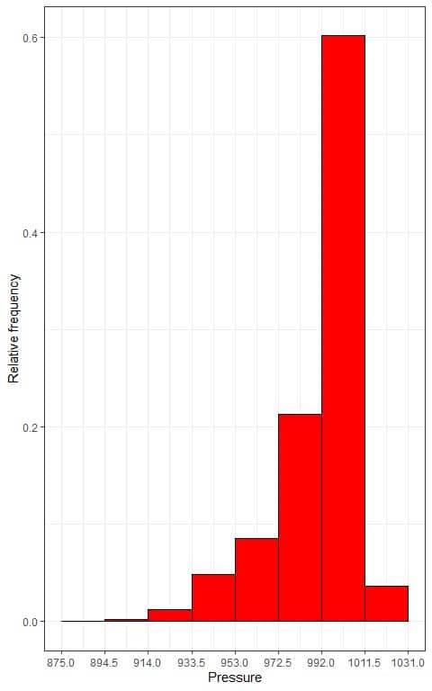
The following frequency table is for the different pressure measurements of 198 tropical storms, measured every six hours during the lifetime of a storm.

The mean = 992 millibars and the standard deviation = 19.5 millibars.

We construct the frequency table by subtracting the standard deviation multiples from the mean or adding the standard deviation multiples to the mean.

Validate Chebyshev’s theorem that:

• At least 75% of the data must lie within 2 standard deviations from the mean.
• At least 88.89% of the data must lie within 3 standard deviations from the mean.

If we sum these frequencies, we will get 10,010 which is the total number of data.

7+ 23+ 124+ 488+ 851+ 2131+ 6023+ 363 = 10010.

1. We add a third column for the relative frequency or probability.

Relative frequency = frequency/total data number.

For example, the first bin contains 7 data points or frequency, so the relative frequency = 7/10010 = 0.001.

If you sum these relative frequencies, you will get 1.

0.001+ 0.002+ 0.012+ 0.049+ 0.085+ 0.213+ 0.602+ 0.036 = 1.

2. We use the table to plot a relative frequency histogram, where the data bins or ranges on the x-axis and the relative frequency or proportions on the y-axis.

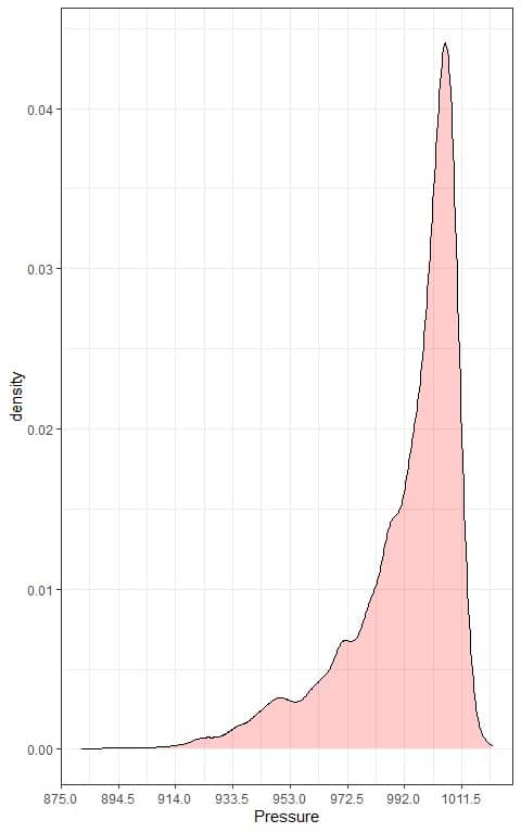
We can also plot a density plot of this data:

3. We can now validate Chebyshev’s theorem that:

• At least 75% of the data must lie within 2 standard deviations from the mean.

The observed proportion for the data within mean +/- (2X standard deviation) = 992 +/- (2X19.5) or within 953 to 1031 = sum of relative frequencies within 953-1031 = 0.085+0.213+0.602+0.036 = 0.936 or 93.6%.

93.6% of our data are within 2 standard deviations from the mean, which is larger than 75%, so this statement is true.

• At least 88.89% of the data must lie within 3 standard deviations from the mean.

The observed proportion for the data within mean +/- (3X standard deviation) = 992 +/- (3X19.5) or within 933.5 to 1050.5 = sum of relative frequencies within 933.5-1050.5 = 0.049+0.085+0.213+0.602+0.036 = 0.985 or 98.5%.

98.5% of our data are within 3 standard deviations from the mean, which is larger than 88.89%, so this statement is true also.

– Example 4

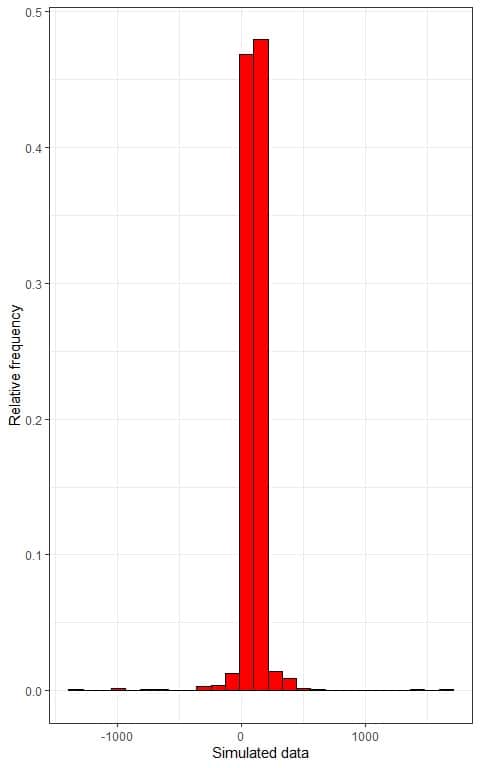
The following frequency table is for 1000 simulated data values.

The mean = 100 and the standard deviation = 115.

The data minimum is -1284.19 and the maximum is 1651.90, so we have many negative bins in this table.

We construct the frequency table by subtracting the standard deviation multiples from the mean or adding the standard deviation multiples to the mean.

Validate Chebyshev’s theorem that:

• At least 75% of the data must lie within 2 standard deviations from the mean
• At least 88.89% of the data must lie within 3 standard deviations from the mean.

If we sum these frequencies, we will get 1000 which is the total number of data.

1. We add a third column for the relative frequency or probability.

Relative frequency = frequency/total data number.

For example, the first bin “-1395 – -1280”contains 1 data point or frequency, so the relative frequency = 1/1000 = 0.001.

If you sum these relative frequencies, you will get 1.

2. We use the table to plot a relative frequency histogram, where the data bins or ranges on the x-axis and the relative frequency or proportions on the y-axis.

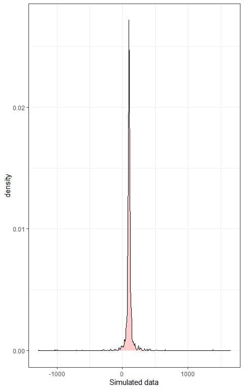
We can also plot a density plot of this data:

3. We can now validate Chebyshev’s theorem that:

• At least 75% of the data must lie within 2 standard deviations from the mean.

The observed proportion for the data within mean +/- (2X standard deviation) = 100 +/- (2X 115) or within -130 to 330 = sum of relative frequencies within -130-330 = 0.013+0.468+0.479+0.014 = 0.974 or 97.4%.

97.4% of our data are within 2 standard deviations from the mean, which is larger than 75%, so this statement is true.

• At least 88.89% of the data must lie within 3 standard deviations from the mean.

The observed proportion for the data within mean +/- (3X standard deviation) = 100 +/- (3X115) or within -245 to 445 = sum of relative frequencies within -245-445 = 0.004+0.013+0.468+0.479+0.014+0.009 = 0.987 or 98.7%.

98.7% of our data are within 3 standard deviations from the mean, which is larger than 88.89%, so this statement is true also.

2. The Chebyshev’s theorem formula

For every numerical data and a real value k > 1, the proportion of data within k standard deviations of the mean is at least:

1-1/k^2

For example, the proportion of data within 2 standard deviations of the mean is at least:

1-1/2^2 =0.75 or 75%.

The proportion of data within 3 standard deviations of the mean is at least:

1-1/3^2 =0.8888 or 88.89%.

Because Chebyshev’s theorem can be applied to any k > 1, we can know the minimum percentage of data that fall within k standard deviation from the mean as shown in the following table:

For example:

• The minimum percentage of data within 1.5 standard deviations from the mean = 55.56%.
• The minimum percentage of data within 2.5 standard deviations from the mean = 84%.
• The minimum percentage of data within 3.5 standard deviations from the mean = 91.84%.

– Example 1

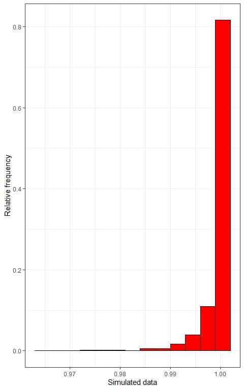
The following frequency table is for 1000 simulated data values from the Beta distribution.

The mean = 0.999 and the standard deviation = 0.003.

The minimum of the data = 0.9643 and the maximum is 1.000.

We construct the frequency table by subtracting the standard deviation multiples from the mean or adding the standard deviation multiples to the mean.

Validate Chebyshev’s theorem that:

• At least 93.75% of the data must lie within 4 standard deviations from the mean.
• At least 96% of the data must lie within 5 standard deviations from the mean.

1. We add a third column for the relative frequency or probability.

Relative frequency = frequency/total data number.

For example, the first bin “0.963-0.966” contains 1 data point or frequency, so the relative frequency = 1/1000 = 0.001.

If you sum these relative frequencies, you will get 1.

2. We use the table to plot a relative frequency histogram, where the data bins or ranges on the x-axis and the relative frequency or proportions on the y-axis:

We can also plot a density plot of this data:

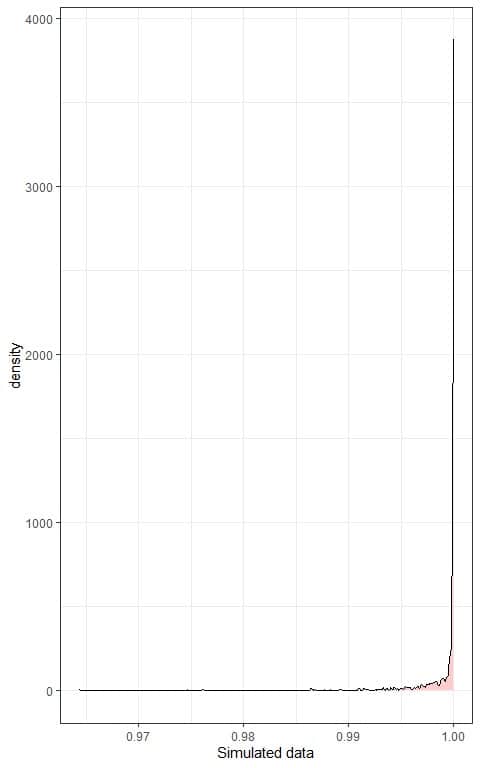
In both plots, we see very left-skewed data.

3. We can now validate Chebyshev’s theorem that:

• At least 93.75% of the data must lie within 4 standard deviations from the mean.

The observed proportion for the data within mean +/- (4X standard deviation) = 0.999 +/- (4X 0.003) or within 0.987 to 1.011 = sum of relative frequencies within 0.987-1.011 = 0.006+0.017+0.039+0.109+0.816 = 0.987 or 98.7%.

98.7% of our data are within 4 standard deviations from the mean, which is larger than 93.75%, so this statement is true.

• At least 96% of the data must lie within 5 standard deviations from the mean.

The observed proportion for the data within mean +/- (5X standard deviation) = 0.999 +/- (5X 0.003) or within 0.984 to 1.014 = sum of relative frequencies within 0.984-1.014 = 0.005+0.006+0.017+0.039+0.109+0.816 = 0.992 or 99.2%.

99.2% of our data are within 5 standard deviations from the mean, which is larger than 96%, so this statement is true also.

3. When to use Chebyshev’s theorem?

Chebyshev’s theorem applies to a distribution with any shape.

However, Chebyshev’s theorem can be used only for k >1.

4. How to use Chebyshev’s theorem?

We use Chebyshev’s theorem to calculate the minimum percentage of data within a certain number of standard deviations from the mean, provided that this number is greater than 1.

– Example 1

The following table is for the areas in thousands of square miles of 48 islands that exceed 10,000 square miles.

The mean = 1253 and the standard deviation = 3371.

The minimum of the areas = 12.0 and the maximum is 16988.0.

What is the minimum percentage of islands that fall within 1.5, 2.5, or 3.5 standard deviations from the mean?

1. The minimum percentage of islands that fall within 1.5 standard deviations from the mean:

1-1/〖1.5〗^2 =0.5555 or 55.56%.

The minimum percentage of islands that fall within 2.5 standard deviations from the mean:

1-1/〖2.5〗^2 =0.84 or 84%.

The minimum percentage of islands that fall within 3.5 standard deviations from the mean:

1-1/〖3.5〗^2 =0.9184 or 91.84%.

2. To show that the results are true, we construct the frequency table for areas by subtracting the standard deviation halves (multiples of 3371/2 = 1685.5) from the mean or adding the standard deviation halves to the mean.

The first bin is a negative 1253-1685.5 = -432.5 so the first bin is 0-1253.

3. We add a third column for the relative frequency or probability.

Relative frequency = frequency/total data number.

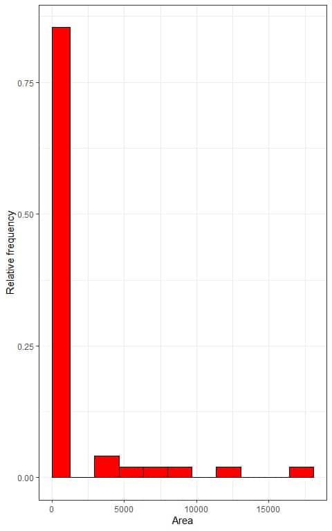
4. We use the table to plot a relative frequency histogram, where the data bins or ranges on the x-axis and the relative frequency or proportions on the y-axis:

We can also plot a density plot of this data:

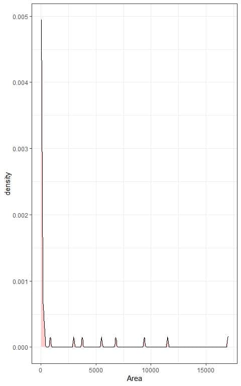
In both plots, we see very right-skewed data.

5. We can now test our results according to Chebyshev’s theorem:

• At least 55.56%. of the data must lie within 1.5 standard deviations from the mean.

The observed proportion for the data within mean +/- (1.5X standard deviation) = 1253 +/- (1.5X 3371) or within 0 to 6309.5 = sum of relative frequencies within 0- 6309.5 = 0.854+0.000+0.042+0.021 = 0.917 or 91.7%.

91.7% of our data are within 1.5 standard deviations from the mean, which is larger than 55.56%, so this result is true.

• At least 84%. of the data must lie within 2.5 standard deviations from the mean.

The observed proportion for the data within mean +/- (2.5X standard deviation) = 1253 +/- (2.5X 3371) or within 0 to 9680.5 = sum of relative frequencies within 0- 9680.5 = 0.854+0.000+0.042+0.021+0.021+0.021 = 0.959 or 95.9%.

95.9% of our data are within 2.5 standard deviation from the mean, which is larger than 84%, so this result is true also.

• At least 91.84% of the data must lie within 3.5 standard deviations from the mean.

The observed proportion for the data within mean +/- (3.5X standard deviation) = 1253 +/- (2.5X 3371) or within 0 to 13051.5 = sum of relative frequencies within 0- 13051.5 = 0.854+0.000+0.042+0.021+0.021+0.021+0.000+0.021 = 0.98 or 98%.

98% of our data are within 3.5 standard deviation from the mean, which is larger than 91.84%, so this result is true also.

5. Practice questions

1. The following histograms are 4 types of simulated data from different distributions.

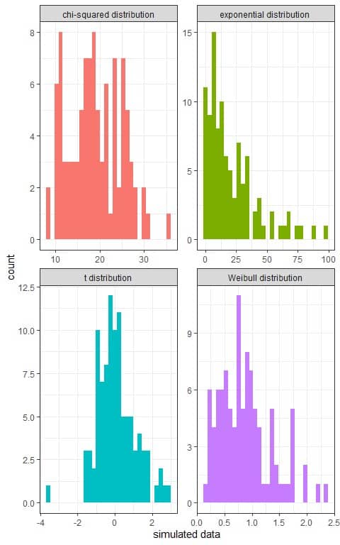
What is the minimum percentage of each data that will fall within 2 standard deviations from the mean?

2. The annual income from a certain mean has a mean = 23,600 USD that is lower than the standard deviation = 46,600 USD.

What is the minimum percentage of this data that will fall between 0 USD and 116,800 USD?

3. The birth weight for a sample of 100 babies has a mean = 120 ounces and standard deviation = 20 ounces.

At least, how many babies from this sample have a birth weight between 90 and 150 ounces?

4. The daily ozone measurement for a sample of 116 days has a mean = 42 ppb and standard deviation = 30 ppb.

At least, how many days from this sample have ozone measurements between 9 and 75 ppb?

5. The daily closing price of the Germany DAX stock index for a sample of 1860 days has a mean = 2530 and standard deviation = 1084.

At least, how many days from this sample have a closing price between 904 and 4156?

6. Answer key

1. Chebyshev’s theorem can be applied to any data from any distribution.

So, the proportion of data within 2 standard deviations of the mean is at least 1-1/2^2 =0.75 or 75%.

2. The maximum limit = 116,800 = mean + 2 X standard deviation = 23600+2X46600.

While mean – 2X standard deviation will be a negative unrealistic number and so can be rounded to 0.

Using Chebyshev’s theorem, the proportion of data within 2 standard deviations of the mean is at least 1-1/2^2 =0.75 or 75%.

3. The limits of 90 and 150 = mean±1.5Xstandarddeviation=120±30.

Using Chebyshev’s theorem, the proportion of data within 1.5 standard deviations of the mean is at least 1-1/〖1.5〗^2 =0.5556 or 55.56%.

As we have 100 babies in our sample, so 100 X 0.55556 = 56 babies approximately.

4. The limits of 9 and 75 = mean±1.1Xstandarddeviation=42±33.

Using Chebyshev’s theorem, the proportion of data within 1.1 standard deviations of the mean is at least 1-1/〖1.1〗^2 =0.1736 or 17.36%.

As we have 116 days in our sample, so 116 X 0.1736 = 20 days at least have ozone measurement between 9 and 75 ppb.

5. The limits of 904 and 4156 = mean±1.5Xstandarddeviation=2530±1626.

Using Chebyshev’s theorem, the proportion of data within 1.5 standard deviations of the mean is at least 1-1/〖1.5〗^2 =0.5556 or 55.56%.

As we have 1860 days in our sample, so 1860 X 0.5556 = 1033 days at least had a daily closing price between 904 and 4156.

Previous Lesson | Main Page | Next Lesson