JUMP TO TOPIC
Chi Square – Explanation & Examples
 The definition of the chi-square test is:
“The chi-square test compares two variables in a contingency table to see if they are related.”
In this topic, we will discuss the chi-square test from the following aspects:
- What is the chi-square test?
- Hypothesis testing using the chi-square test.
- Steps of hypothesis testing performed by the chi-square test.
- How to calculate the chi-square test?
- Practice questions.
- Answer key.
1. What is the chi-square test?
The chi-square test of independence, also called χ^2 test, is used to analyze the contingency table formed by two categorical variables.
The chi-square test evaluates whether there is a significant association between the categories of the two variables.
An R × C contingency table is a table with R rows and C columns. It displays the relationship between two variables, where the variable in the rows has R categories and the variable in the columns has C categories.
– Example of 2 X 2 contingency table
A study in 1994 examined 491 dogs that had developed cancer and 945 dogs as a control group (without cancer) to determine whether there is an increased risk of cancer in dogs that are exposed to the herbicide 2,4-Dichlorophenoxyacetic acid (2,4-D).
Reference:
Hayes HM, Tarone RE, Cantor KP, Jessen CR, McCurnin DM, and Richardson RC. 1991. Case-Control Study of Canine Malignant Lymphoma: Positive Association With Dog Owner’s Use of 2, 4- Dichlorophenoxyacetic Acid Herbicides. Journal of the National Cancer Institute 83(17):1226-1231.
The results of this study are shown in the following table.
| cancer | no cancer | Sum |
2,4-D | 191 | 304 | 495 |
no 2,4-D | 300 | 641 | 941 |
Sum | 491 | 945 | 1436 |
We see that:
- The 2,4-D exposure categories are indicated along the rows and the cancer status categories are indicated along with the columns.
- The data are arranged in the form of a 2 × 2 contingency table because the 2,4-D exposure has 2 categories and the cancer status has 2 categories also.
- The “cancer” and “no cancer” columns for dogs that developed and did not develop cancer respectively.
- The “2,4-D” and “no 2,4-D” rows for dogs that were exposed and were not exposed to 2,4-D respectively.
- 191 dogs were exposed to 2,4-D and developed cancer.
- 304 dogs were exposed to 2,4-D and did not develop cancer.
- 300 dogs were not exposed to 2,4-D and developed cancer.
- 641 dogs were not exposed to 2,4-D and did not develop cancer.
We want to test for the relationship between exposure to 2,4-D and developing cancer. We use the χ^2 test to test if this relationship truly exists.
– Example of 2 X 5 contingency table
Survey responses for 20,000 responses to the Behavioral Risk Factor Surveillance System.
Source Office of Surveillance, Epidemiology, and Laboratory Services Behavioral Risk Factor Surveillance System, BRFSS 2010 Survey Data.
The results of this study are shown in the following table.
| Excellent | Fair | Good | Poor | Very good | Sum |
No | 459 | 385 | 854 | 99 | 727 | 2524 |
Yes | 4198 | 1634 | 4821 | 578 | 6245 | 17476 |
Sum | 4657 | 2019 | 5675 | 677 | 6972 | 20000 |
We see that:
- The health coverage categories are indicated along the rows and the health status categories are indicated along with the columns.
- The data are arranged in the form of a 2 × 5 contingency table because the health coverage has 2 categories and the health status has 5 categories.
- The “Excellent”, “Fair”, “Good”, “Poor”, and “Very good” columns are for the person’s health status.
- The “No” and “Yes” rows are for whether the person had health coverage or not.
- 459 persons had excellent health status and were not having health coverage.
- 4198 persons had excellent health status and were having health coverage.
- 385 persons had fair health status and were not having health coverage.
- 1634 persons had fair health status and were having health coverage.
- 854 persons had good health status and were not having health coverage.
- 4821 persons had good health status and were having health coverage.
- 99 persons had poor health status and were not having health coverage.
- 578 persons had poor health status and were having health coverage.
- 727 persons had very good health status and were not having health coverage.
- 6245 persons had very good health status and were having health coverage.
We want to test for the relationship between health status and health coverage. We use the χ^2 test to test if this relationship truly exists.
– Example of 4 X 3 contingency table
A 2010 Pew Research poll asked 1,306 Americans, “From what you’ve read and heard, is there solid evidence that the average temperature on earth has been getting warmer over the past few decades, or not?”
Source: Pew Research Center, Majority of Republicans No Longer See Evidence of Global Warming, data collected on October 27, 2010.
The results of this study are shown in the following table.
| Don’t know / refuse to answer | Earth is warming | Not warming | Sum |
Conservative Republican | 45 | 248 | 450 | 743 |
Liberal Democrat | 23 | 405 | 23 | 451 |
Mod/Cons Democrat | 45 | 563 | 158 | 766 |
Mod/Lib Republican | 23 | 135 | 135 | 293 |
Sum | 136 | 1351 | 766 | 2253 |
We see that:
- The party categories are indicated along the rows and the response categories are indicated along with the columns.
- The data are arranged in the form of a 4 × 3 contingency table because the party has 4 categories and the response has 3 categories.
- The “Don’t know / refuse to answer”, “Earth is warming”, and “Not warming” columns are the response categories.
- The “Conservative Republican”, “Liberal Democrat”, “Mod/Cons Democrat”, and “Mod/Lib Republican” rows are the party categories.
- 45 persons responded “Don’t know / refuse to answer” and were having “Conservative Republican” party, compared to 23 persons having “Liberal Democrat” party, 45 persons having “Mod/Cons Democrat” party, and 23 persons having “Mod/Lib Republican” party.
- 248 persons responded “Earth is warming” and were having “Conservative Republican” party, compared to 405 persons having “Liberal Democrat” party,
- 563 persons having “Mod/Cons Democrat” party, and 135 persons having “Mod/Lib Republican” party.
- 450 persons responded “Not warming” and were having “Conservative Republican” party, compared to 23 persons having “Liberal Democrat” party,
- 158 persons having “Mod/Cons Democrat” party, and 135 persons having “Mod/Lib Republican” party.
We want to test for the relation between the party categories and the response categories. We use the χ^2 test to test if this relationship truly exists.
2. Hypothesis testing using the chi-square test
Where you start with two exclusive possibilities for the unknown truth. Then, use the sample to choose between these two possibilities for the truth. The two possibilities are the Null hypothesis, Ho, and the Alternative hypothesis, Ha.
- The null hypothesis, Ho: There is no difference between the two populations or the two categorical variables, and the difference = zero.
- The alternative hypothesis, Ha: There is a difference between the two populations so the difference ≠ zero.
Hypothesis testing is denoted as:
- Ho: p_1=p_2 or p_1-p_2=0. The proportions of one variable are the same for different values of the other variable.
In testing the relation between exposure to 2,4-D and developing cancer, this means that the proportion of developing cancer is similar for dogs exposed and not exposed to 2,4-D.
- Ha: p_1≠p_2 or p_1-p_2≠0. In testing the relation between exposure to 2,4-D and developing cancer, this means that the proportion of developing cancer is different for dogs exposed and not exposed to 2,4-D.
Note: Although the hypothesis testing for the chi-square test compares proportions, the chi-square test uses the actual count to test that.
– Steps of hypothesis testing performed by the chi-square test
- The chi-square test uses the contingency table of data to calculate an expected table.
The expected table contains the theoretical data counts that would be expected when there is no relation between the rows and the columns i.e. the null hypothesis is true, Ho: p_1=p_2.
- The test calculates the discrepancies between each observed and expected value and aggregates them.
- If the null hypothesis is true, the aggregated value, called the χ^2 statistic, has a chi-square distribution. Define the probability of the aggregated value under this chi-square distribution. This is the p-value.
The p-value is the probability of our sample results if the null hypothesis is true.
The null hypothesis means that the proportion of developing cancer is similar for dogs exposed and not exposed to 2,4-D.
Generally in research, the cut-off used is 0.05. This 0.05 is called the rejection level, α level, or significance level.
- Make a decision, accept Ha, or fail to reject Ho.
If p-value < 0.05, so it is a statistically significant result at 0.05 level. Reject the null hypothesis and conclude that our sample data are unlikely under the Ho, null hypothesis, they have a probability of less than 0.05.
If p-value >= 0.05, so it is a statistically non-significant result at 0.05 level and we fail to reject the Null hypothesis.
We say fail to reject the Null hypothesis because if we have a p-value of 0.25. This means that our sample data have a probability of 25% under the null hypothesis which is considered a large percentage. In your opinion, you may consider it small and accept Ha.
Note: No expected value in the expected table is less than 5 (sometimes known as “the rule of five”). If any expected value is less than 5, the chi-square test is not applicable and other tests are applied (Fisher Exact test).
3. How to calculate the chi-square test?
– Example of 2 X 2 contingency table
A study in 1994 examined 491 dogs that had developed cancer and 945 dogs as a control group to determine whether there is an increased risk of cancer in dogs that are exposed to the herbicide 2,4-Dichlorophenoxyacetic acid (2,4-D).
The following 2 X 2 contingency table is obtained:
| cancer | no cancer | Sum |
2,4-D | 191 | 304 | 495 |
no 2,4-D | 300 | 641 | 941 |
Sum | 491 | 945 | 1436 |
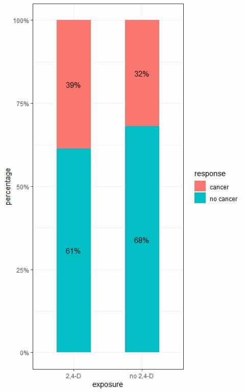
To see the different proportions of cancer development per 2,4-D exposure, we can use the following table:
| cancer | no cancer |
2,4-D | 0.39 | 0.61 |
no 2,4-D | 0.32 | 0.68 |
The sum of every row is 1.00 or 100%.
We see that 0.39 or 39% of dogs exposed to 2,4-D developed cancer compared to 0.32 or 32% of dogs not exposed to 2,4-D.
We can plot these proportions in the following bar plot.
To test for the relationship between exposure to 2,4-D and developing cancer, we follow these steps:
- Use the 2 X 2 table to calculate the expected count of each cell.
The expected count in the (i, j) cell =
(the total count in the ith row X the total count in the jth column)/ the total count in the table.
The expected counts indicate no association between the rows and columns. In other words, there is no association between exposure to 2,4-D and cancer development.
The sum of the expected values across any row or column must equal the corresponding row or column total.
The expected count for dogs exposed to 2,4-D and developed cancer = (total in 1st row X total in 1st column)/table total = (495X491)/1436 = 169.2514.
The expected count for dogs not exposed to 2,4-D and developed cancer = (total in 2nd row X total in 1st column)/table total = (941X491)/1436 = 321.7486.
The expected count for dogs exposed to 2,4-D and did not develop cancer = (total in 1st row X total in 2nd column)/table total = (495X945)/1436 = 325.7486.
The expected count for dogs not exposed to 2,4-D and did not develop cancer = (total in 2nd row X total in 2nd column)/table total = (941X945)/1436 = 619.2514.
The following table will be produced:
| cancer | no cancer | Sum |
2,4-D | 169.2514 | 325.7486 | 495 |
no 2,4-D | 321.7486 | 619.2514 | 941 |
Sum | 491.0000 | 945.0000 | 1436 |
We see that all expected values are larger than 5 so the chi-square test can be used.
To see the different proportions of cancer development per 2,4-D exposure in the expected table:
| cancer | no cancer |
2,4-D | 0.34 | 0.66 |
no 2,4-D | 0.34 | 0.66 |
The sum of every row is 1.00 or 100%.
We see that 0.34 or 34% of dogs exposed to 2,4-D developed cancer and also 0.34 or 34% of dogs not exposed to 2,4-D.
- Make a table with 2 columns for different cells and their observed counts.
We have 4 cells in this 2 X 2 table:
- A cell for dogs exposed to 2,4-D and had cancer.
- A cell for dogs exposed to 2,4-D and had not cancer.
- A cell for dogs not exposed to 2,4-D and had cancer.
- A cell for dogs not exposed to 2,4-D and had not cancer.
category | observed |
2,4-D, cancer | 191 |
no 2,4-D,cancer | 300 |
2,4-D,no cancer | 304 |
no 2,4-D, no cancer | 641 |
- Add a column for the expected count of each cell.
category | observed | expected |
2,4-D,cancer | 191 | 169.2514 |
no 2,4-D,cancer | 300 | 321.7486 |
2,4-D,no cancer | 304 | 325.7486 |
no 2,4-D,no cancer | 641 | 619.2514 |
- Subtract the expected value from the Observed value and place the result in the “obs-exp” column.
category | observed | expected | obs-exp |
2,4-D,cancer | 191 | 169.2514 | 21.75 |
no 2,4-D,cancer | 300 | 321.7486 | -21.75 |
2,4-D,no cancer | 304 | 325.7486 | -21.75 |
no 2,4-D,no cancer | 641 | 619.2514 | 21.75 |
- Square the differences from Step 4 and place the result in the “(obs-exp)^2” column.
category | observed | expected | obs-exp | (obs-exp)^2 |
2,4-D, cancer | 191 | 169.2514 | 21.75 | 473.06 |
no 2,4-D,cancer | 300 | 321.7486 | -21.75 | 473.06 |
2,4-D,no cancer | 304 | 325.7486 | -21.75 | 473.06 |
no 2,4-D,no cancer | 641 | 619.2514 | 21.75 | 473.06 |
- Divide the squared differences by their respective expected value and place the result in the “(obs-exp)^2/exp” column.
category | observed | expected | obs-exp | (obs-exp)^2 | (obs-exp)^2/exp |
2,4-D,cancer | 191 | 169.2514 | 21.75 | 473.06 | 2.80 |
no 2,4-D,cancer | 300 | 321.7486 | -21.75 | 473.06 | 1.47 |
2,4-D,no cancer | 304 | 325.7486 | -21.75 | 473.06 | 1.45 |
no 2,4-D,no cancer | 641 | 619.2514 | 21.75 | 473.06 | 0.76 |
- Sum all the values in the last column to get the chi-square statistic:
The χ^2 statistic = 2.80+1.47+1.45+0.76 = 6.48.
The last column is summed to get an overall measure of agreement between the observed and expected tables.
- If the null hypothesis is true, the χ^2 statistic has a chi-square distribution with (R − 1) × (C − 1) degrees of freedom or df.
Define the probability (or the p-value) of the χ^2 statistic under this chi-square distribution.
The p-value is given by the area to the right of the χ^2 statistic under this chi-square distribution.
In our 2X2 contingency table, the df = (2-1)X(2-1) = 1.
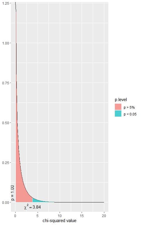
The following is the chi-square distribution with 1 df.

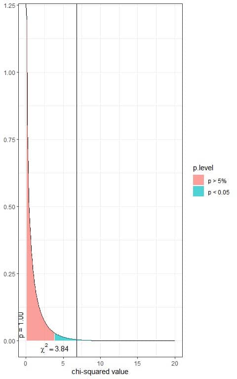
The total area under the curve is 1.00 or 100%.
In the first plot, we see that when the χ^2 value = 3.84, the area to the right or the p-value = 0.05.
In our contingency table, the χ^2 value = 6.84 (plotted as a vertical line in the second plot), so the p-value is smaller than 0.05.
- Make a decision, accept Ha, or fail to reject Ho.
The p-value < 0.05, so it is a statistically significant result. We reject the null hypothesis and conclude that our sample data are unlikely under the Ho, null hypothesis, they have a probability of less than 0.05.
We conclude that there is a significant relationship between exposure to 2,4-D and cancer development in dogs.
– Example of 2 X 5 contingency table
The Survey responses for 20,000 responses to the Behavioral Risk Factor Surveillance System.
The results of this study are shown in the following table.
| Excellent | Fair | Good | Poor | Very good | Sum |
No | 459 | 385 | 854 | 99 | 727 | 2524 |
Yes | 4198 | 1634 | 4821 | 578 | 6245 | 17476 |
Sum | 4657 | 2019 | 5675 | 677 | 6972 | 20000 |
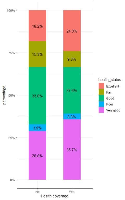
To see the different proportions of health status per health coverage, we can use the following table:
| Excellent | Fair | Good | Poor | Very good |
No | 0.18 | 0.15 | 0.34 | 0.04 | 0.29 |
Yes | 0.24 | 0.09 | 0.28 | 0.03 | 0.36 |
The sum of every row is 1.00 or 100%.
We see that 0.18 or 18% of persons who do not have health coverage had excellent health status compared to 0.24 or 24% of persons who do have health coverage.
We see that 0.15 or 15% of persons who do not have health coverage had fair health status compared to 0.09 or 9% of persons who do have health coverage, and so on.
We can plot these proportions in the following bar plot.
To test for the relationship between health coverage and health status, we follow these steps:
- Use the 2 X 5 table to calculate the expected count of each cell.
The expected counts indicate no association between the rows and columns. In other words, there is no association between health coverage and health status.
The expected count in the (i, j) cell =
(the total count in the ith row X the total count in the jth column)/ the total count in the table.
For example, the expected count for persons who do not have a health coverage and with excellent health status = (row total X column total) / table total = (2524 X 4657)/20000 = 587.7134.
The following table will be produced:
| Excellent | Fair | Good | Poor | Very good | Sum |
No | 587.7134 | 254.7978 | 716.185 | 85.4374 | 879.8664 | 2524 |
Yes | 4069.2866 | 1764.2022 | 4958.815 | 591.5626 | 6092.1336 | 17476 |
Sum | 4657.0000 | 2019.0000 | 5675.000 | 677.0000 | 6972.0000 | 20000 |
We see that all expected values are larger than 5 so the chi-square test can be used.
To see the different proportions of health statuses per health coverage in the expected table:
| Excellent | Fair | Good | Poor | Very good |
No | 0.23 | 0.1 | 0.28 | 0.03 | 0.35 |
Yes | 0.23 | 0.1 | 0.28 | 0.03 | 0.35 |
We see that 0.23 or 23% of persons who do or do not have health coverage had excellent health status.
All other proportions of different health statuses across the health coverage are equal.
- Make a table with 2 columns for different cells and their observed counts.
We have 10 cells in this 2 X 5 table which are shown in the following table:
category | observed |
No, Excellent | 459 |
Yes, Excellent | 4198 |
No, Fair | 385 |
Yes, Fair | 1634 |
No, Good | 854 |
Yes, Good | 4821 |
No, Poor | 99 |
Yes, Poor | 578 |
No, Very good | 727 |
Yes, Very good | 6245 |
For example, the “No, Excellent” category means persons without health coverage and excellent health status.
- Add a column for the expected count of each cell.
category | observed | expected |
No, Excellent | 459 | 587.7134 |
Yes, Excellent | 4198 | 4069.2866 |
No, Fair | 385 | 254.7978 |
Yes, Fair | 1634 | 1764.2022 |
No, Good | 854 | 716.1850 |
Yes, Good | 4821 | 4958.8150 |
No,Poor | 99 | 85.4374 |
Yes, Poor | 578 | 591.5626 |
No, Very good | 727 | 879.8664 |
Yes, Very good | 6245 | 6092.1336 |
- Subtract the expected value from the Observed value and place the result in the “obs-exp” column.
category | observed | expected | obs-exp |
No,Excellent | 459 | 587.7134 | -128.71 |
Yes,Excellent | 4198 | 4069.2866 | 128.71 |
No,Fair | 385 | 254.7978 | 130.20 |
Yes,Fair | 1634 | 1764.2022 | -130.20 |
No,Good | 854 | 716.1850 | 137.82 |
Yes,Good | 4821 | 4958.8150 | -137.81 |
No,Poor | 99 | 85.4374 | 13.56 |
Yes,Poor | 578 | 591.5626 | -13.56 |
No,Very good | 727 | 879.8664 | -152.87 |
Yes, Very good | 6245 | 6092.1336 | 152.87 |
- Square the differences from Step 4 and place the result in the “(obs-exp)^2” column.
category | observed | expected | obs-exp | (obs-exp)^2 |
No,Excellent | 459 | 587.7134 | -128.71 | 16566.26 |
Yes,Excellent | 4198 | 4069.2866 | 128.71 | 16566.26 |
No,Fair | 385 | 254.7978 | 130.20 | 16952.04 |
Yes,Fair | 1634 | 1764.2022 | -130.20 | 16952.04 |
No,Good | 854 | 716.1850 | 137.82 | 18994.35 |
Yes,Good | 4821 | 4958.8150 | -137.81 | 18991.60 |
No,Poor | 99 | 85.4374 | 13.56 | 183.87 |
Yes,Poor | 578 | 591.5626 | -13.56 | 183.87 |
No,Very good | 727 | 879.8664 | -152.87 | 23369.24 |
Yes,Very good | 6245 | 6092.1336 | 152.87 | 23369.24 |
- Divide the squared differences by their respective expected value and place the result in the “(obs-exp)^2/exp” column.
category | observed | expected | obs-exp | (obs-exp)^2 | (obs-exp)^2/exp |
No,Excellent | 459 | 587.7134 | -128.71 | 16566.26 | 28.19 |
Yes,Excellent | 4198 | 4069.2866 | 128.71 | 16566.26 | 4.07 |
No,Fair | 385 | 254.7978 | 130.20 | 16952.04 | 66.53 |
Yes,Fair | 1634 | 1764.2022 | -130.20 | 16952.04 | 9.61 |
No,Good | 854 | 716.1850 | 137.82 | 18994.35 | 26.52 |
Yes,Good | 4821 | 4958.8150 | -137.81 | 18991.60 | 3.83 |
No,Poor | 99 | 85.4374 | 13.56 | 183.87 | 2.15 |
Yes,Poor | 578 | 591.5626 | -13.56 | 183.87 | 0.31 |
No,Very good | 727 | 879.8664 | -152.87 | 23369.24 | 26.56 |
Yes,Very good | 6245 | 6092.1336 | 152.87 | 23369.24 | 3.84 |
- Sum all the values in the last column to get the chi-square statistic:
The χ^2 statistic = 28.19+ 4.07+ 66.53+ 9.61+ 26.52+ 3.83+ 2.15+ 0.31+ 26.56+ 3.84 = 171.61.
- If the null hypothesis is true, the χ^2 statistic has a chi-square distribution with (R − 1) × (C − 1) degrees of freedom.
In our 2X5 contingency table, the df = (2-1)X(5-1) = 4.
The following is the chi-square distribution with 4 df.
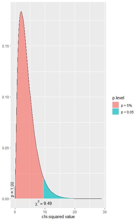
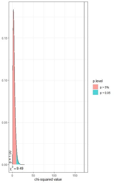
In the first plot, we see that when the χ^2 value = 9.49, the area to the right or the p-value = 0.05.
In our contingency table, the χ^2 value = 171.61 (plotted as a vertical line in the second plot), so the p-value is very much smaller than 0.05.
- Make a decision, accept Ha, or fail to reject Ho.
The p-value < 0.05, so it is a statistically significant result. We reject the null hypothesis and conclude that our sample data are unlikely under the Ho or the null hypothesis.
We conclude that there is a significant relationship between health statuses and health coverage in the persons surveyed.
– Example of 4 X 3 contingency table
A 2010 Pew Research poll asked 1,306 Americans, “From what you’ve read and heard, is there solid evidence that the average temperature on earth has been getting warmer over the past few decades, or not?”.
The results of this study are shown in the following table.
| Don’t know / refuse to answer | Earth is warming | Not warming | Sum |
Conservative Republican | 45 | 248 | 450 | 743 |
Liberal Democrat | 23 | 405 | 23 | 451 |
Mod/Cons Democrat | 45 | 563 | 158 | 766 |
Mod/Lib Republican | 23 | 135 | 135 | 293 |
Sum | 136 | 1351 | 766 | 2253 |
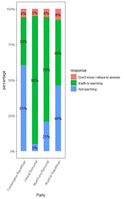
To see the different proportions of responses per different parties, we can use the following table:
| Don’t know / refuse to answer | Earth is warming | Not warming |
Conservative Republican | 0.06 | 0.33 | 0.61 |
Liberal Democrat | 0.05 | 0.90 | 0.05 |
Mod/Cons Democrat | 0.06 | 0.73 | 0.21 |
Mod/Lib Republican | 0.08 | 0.46 | 0.46 |
The sum of every row is 1.00 or 100%.
We see that:
- 0.33 or 33% of “Conservative Republican” persons responded that Earth is warming, compared to 0.90 or 90% of “Liberal Democrat” persons, 0.73 or 73% of “Mod/Cons Democrat” persons, and 0.46 or 46% of “Mod/Lib Republican” persons.
- 0.61 or 61% of “Conservative Republican” persons responded that Earth is not warming, compared to only 0.05 or 5% of “Liberal Democrat” persons, 0.21 or 21% of “Mod/Cons Democrat” persons, and 0.46 or 46% of “Mod/Lib Republican” persons.
We can plot these proportions in the following bar plot.
To test for the relationship between parties and responses, we follow these steps:
- Use the 4 X 3 table to calculate the expected count of each cell.
The expected counts indicate no association between the rows and columns. In other words, there is no association between the parties and the responses.
The expected count in the (i, j) cell =
(the total count in the ith row X the total count in the jth column)/ the total count in the table.
For example, the expected count for “Conservative Republican” persons who responded that Earth is warming = (row total X column total) / table total = (743 X 1351)/2253 = 445.5362.
The following table will be produced:
| Don’t know / refuse to answer | Earth is warming | Not warming | Sum |
Conservative Republican | 44.85042 | 445.5362 | 252.6134 | 743 |
Liberal Democrat | 27.22415 | 270.4399 | 153.3360 | 451 |
Mod/Cons Democrat | 46.23879 | 459.3280 | 260.4332 | 766 |
Mod/Lib Republican | 17.68664 | 175.6960 | 99.6174 | 293 |
Sum | 136.00000 | 1351.0000 | 766.0000 | 2253 |
We see that all expected values are larger than 5 so the chi-square test can be used.
To see the different proportions of responses per parties in the expected table:
| Don’t know / refuse to answer | Earth is warming | Not warming |
Conservative Republican | 0.06 | 0.6 | 0.34 |
Liberal Democrat | 0.06 | 0.6 | 0.34 |
Mod/Cons Democrat | 0.06 | 0.6 | 0.34 |
Mod/Lib Republican | 0.06 | 0.6 | 0.34 |
All proportions of different responses across the different parties are the same.
- Make a table with 2 columns for different cells and their observed counts.
We have 12 cells in this 4 X 3 table which are shown in the following table:
category | observed |
Conservative Republican,Don’t know / refuse to answer | 45 |
Liberal Democrat,Don’t know / refuse to answer | 23 |
Mod/Cons Democrat,Don’t know / refuse to answer | 45 |
Mod/Lib Republican,Don’t know / refuse to answer | 23 |
Conservative Republican,Earth is warming | 248 |
Liberal Democrat,Earth is warming | 405 |
Mod/Cons Democrat,Earth is warming | 563 |
Mod/Lib Republican,Earth is warming | 135 |
Conservative Republican,Not warming | 450 |
Liberal Democrat,Not warming | 23 |
Mod/Cons Democrat,Not warming | 158 |
Mod/Lib Republican,Not warming | 135 |
For example, the “Conservative Republican,Earth is warming” category means “Conservative Republican” persons who responded that Earth is warming.
- Add a column for the expected count of each cell.
category | observed | expected |
Conservative Republican,Don’t know / refuse to answer | 45 | 44.85042 |
Liberal Democrat,Don’t know / refuse to answer | 23 | 27.22415 |
Mod/Cons Democrat,Don’t know / refuse to answer | 45 | 46.23879 |
Mod/Lib Republican,Don’t know / refuse to answer | 23 | 17.68664 |
Conservative Republican,Earth is warming | 248 | 445.53617 |
Liberal Democrat,Earth is warming | 405 | 270.43986 |
Mod/Cons Democrat,Earth is warming | 563 | 459.32801 |
Mod/Lib Republican,Earth is warming | 135 | 175.69596 |
Conservative Republican,Not warming | 450 | 252.61340 |
Liberal Democrat,Not warming | 23 | 153.33600 |
Mod/Cons Democrat,Not warming | 158 | 260.43320 |
Mod/Lib Republican,Not warming | 135 | 99.61740 |
- Subtract the expected value from the Observed value and place the result in the “obs-exp” column.
category | observed | expected | obs-exp |
Conservative Republican,Don’t know / refuse to answer | 45 | 44.85042 | 0.15 |
Liberal Democrat,Don’t know / refuse to answer | 23 | 27.22415 | -4.22 |
Mod/Cons Democrat,Don’t know / refuse to answer | 45 | 46.23879 | -1.24 |
Mod/Lib Republican,Don’t know / refuse to answer | 23 | 17.68664 | 5.31 |
Conservative Republican,Earth is warming | 248 | 445.53617 | -197.54 |
Liberal Democrat,Earth is warming | 405 | 270.43986 | 134.56 |
Mod/Cons Democrat,Earth is warming | 563 | 459.32801 | 103.67 |
Mod/Lib Republican,Earth is warming | 135 | 175.69596 | -40.70 |
Conservative Republican,Not warming | 450 | 252.61340 | 197.39 |
Liberal Democrat,Not warming | 23 | 153.33600 | -130.34 |
Mod/Cons Democrat,Not warming | 158 | 260.43320 | -102.43 |
Mod/Lib Republican,Not warming | 135 | 99.61740 | 35.38 |
- Square the differences from Step 4 and place the result in the “(obs-exp)^2” column.
category | observed | expected | obs-exp | (obs-exp)^2 |
Conservative Republican,Don’t know / refuse to answer | 45 | 44.85042 | 0.15 | 0.02 |
Liberal Democrat,Don’t know / refuse to answer | 23 | 27.22415 | -4.22 | 17.81 |
Mod/Cons Democrat,Don’t know / refuse to answer | 45 | 46.23879 | -1.24 | 1.54 |
Mod/Lib Republican,Don’t know / refuse to answer | 23 | 17.68664 | 5.31 | 28.20 |
Conservative Republican,Earth is warming | 248 | 445.53617 | -197.54 | 39022.05 |
Liberal Democrat,Earth is warming | 405 | 270.43986 | 134.56 | 18106.39 |
Mod/Cons Democrat,Earth is warming | 563 | 459.32801 | 103.67 | 10747.47 |
Mod/Lib Republican,Earth is warming | 135 | 175.69596 | -40.70 | 1656.49 |
Conservative Republican,Not warming | 450 | 252.61340 | 197.39 | 38962.81 |
Liberal Democrat,Not warming | 23 | 153.33600 | -130.34 | 16988.52 |
Mod/Cons Democrat,Not warming | 158 | 260.43320 | -102.43 | 10491.90 |
Mod/Lib Republican,Not warming | 135 | 99.61740 | 35.38 | 1251.74 |
- Divide the squared differences by their respective expected value and place the result in the “(obs-exp)^2/exp” column.
category | observed | expected | obs-exp | (obs-exp)^2 | (obs-exp)^2/exp |
Conservative Republican,Don’t know / refuse to answer | 45 | 44.85042 | 0.15 | 0.02 | 0.00 |
Liberal Democrat,Don’t know / refuse to answer | 23 | 27.22415 | -4.22 | 17.81 | 0.65 |
Mod/Cons Democrat,Don’t know / refuse to answer | 45 | 46.23879 | -1.24 | 1.54 | 0.03 |
Mod/Lib Republican,Don’t know / refuse to answer | 23 | 17.68664 | 5.31 | 28.20 | 1.59 |
Conservative Republican,Earth is warming | 248 | 445.53617 | -197.54 | 39022.05 | 87.58 |
Liberal Democrat,Earth is warming | 405 | 270.43986 | 134.56 | 18106.39 | 66.95 |
Mod/Cons Democrat,Earth is warming | 563 | 459.32801 | 103.67 | 10747.47 | 23.40 |
Mod/Lib Republican,Earth is warming | 135 | 175.69596 | -40.70 | 1656.49 | 9.43 |
Conservative Republican,Not warming | 450 | 252.61340 | 197.39 | 38962.81 | 154.24 |
Liberal Democrat,Not warming | 23 | 153.33600 | -130.34 | 16988.52 | 110.79 |
Mod/Cons Democrat,Not warming | 158 | 260.43320 | -102.43 | 10491.90 | 40.29 |
Mod/Lib Republican,Not warming | 135 | 99.61740 | 35.38 | 1251.74 | 12.57 |
- Sum all the values in the last column to get the chi-square statistic:
The χ^2 statistic = 507.52.
- If the null hypothesis is true, the χ^2 statistic has a chi-square distribution with (R − 1) × (C − 1) degrees of freedom.
In our 4X3 contingency table, the df = (4-1)X(3-1) = 6.
The following is the chi-square distribution with 6 df.
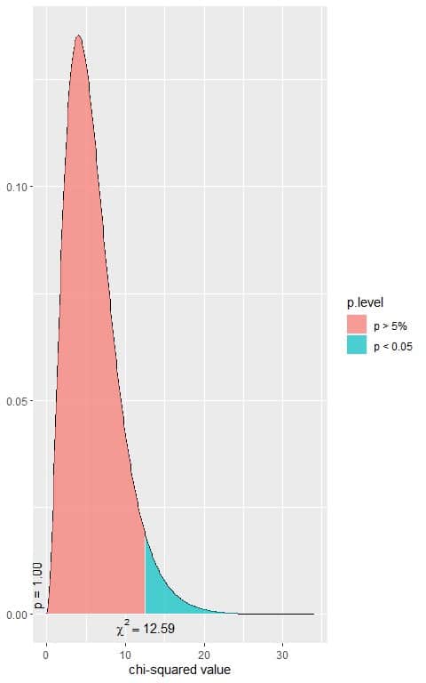
In the first plot, we see that when the χ^2 value = 12.59, the area to the right or the p-value = 0.05.
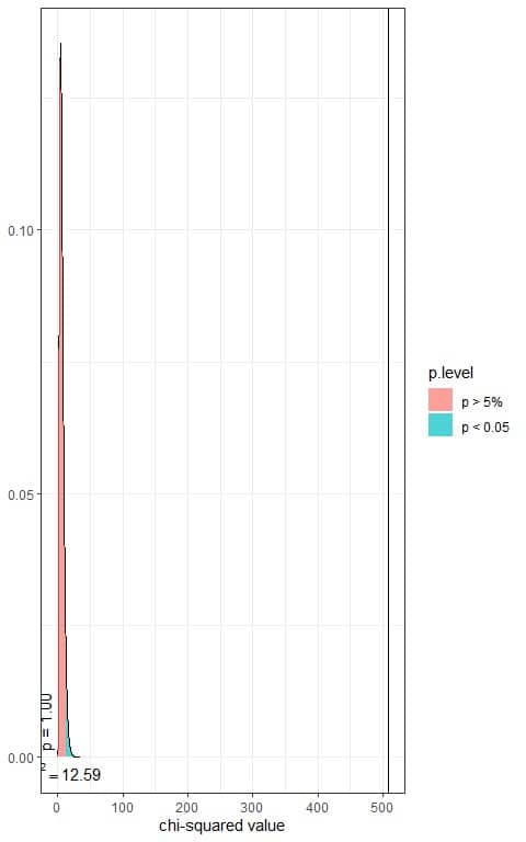
In our contingency table, the χ^2 value = 507.52 (plotted as a vertical line in the second plot), so the p-value is very much smaller than 0.05.
- Make a decision, accept Ha, or fail to reject Ho.
The p-value < 0.05, so it is a statistically significant result. We reject the null hypothesis and conclude that our sample data are unlikely under the null hypothesis.
We conclude that there is a significant relationship between the different parties and the response type in the persons surveyed.
5. Practice questions
1. The Data from the 2010 General Social Survey shows the following table.
| LEGAL | NOT LEGAL | Sum |
BACHELOR | 119 | 112 | 231 |
GRADUATE | 73 | 63 | 136 |
HIGH SCHOOL | 304 | 307 | 611 |
JUNIOR COLLEGE | 42 | 44 | 86 |
LT HIGH SCHOOL | 65 | 130 | 195 |
Sum | 603 | 656 | 1259 |
The rows are for the educational degree and the columns for answering the question “Do you think the use of marijuana should be made legal, or not?”.
Is there a relationship between educational degree and the answer type?
2. A sample of categorical variables from the General Social survey showed the following table.
| Other | Black | White | Sum |
$25000 or more | 621 | 886 | 5856 | 7363 |
$20000 – 24999 | 112 | 220 | 951 | 1283 |
$15000 – 19999 | 134 | 180 | 734 | 1048 |
$10000 – 14999 | 126 | 210 | 832 | 1168 |
$8000 to 9999 | 41 | 56 | 243 | 340 |
$7000 to 7999 | 24 | 27 | 137 | 188 |
$6000 to 6999 | 26 | 35 | 154 | 215 |
$5000 to 5999 | 27 | 40 | 160 | 227 |
$4000 to 4999 | 34 | 38 | 154 | 226 |
$3000 to 3999 | 35 | 59 | 182 | 276 |
$1000 to 2999 | 47 | 71 | 277 | 395 |
Lt $1000 | 36 | 51 | 199 | 286 |
Sum | 1263 | 1873 | 9879 | 13015 |
The rows are for the reported income and the columns for race categories.
Is there a relationship between race and the reported income?
3. A study from the 1970s about whether gender influences hiring recommendations showed the following table.
| not | promoted | Sum |
female | 10 | 14 | 24 |
male | 3 | 21 | 24 |
Sum | 13 | 35 | 48 |
The rows are for the gender and the columns for the promotions.
All expected values are larger than 5 so the chi-square test can be used.
The χ^2 statistic = 5.1692.
The following is the chi-square distribution with 1 df.
Is that a significant result?
4. The demographic information on every member of a 1000 random sample of the US armed forces showed the following table.
| female | male | Sum |
air force | 40 | 175 | 215 |
army | 54 | 351 | 405 |
marine corps | 6 | 148 | 154 |
navy | 34 | 192 | 226 |
Sum | 134 | 866 | 1000 |
The rows are for the branch of the armed forces: air force, army, marine corps, or navy, and the columns for the gender.
All expected values are larger than 5 so the chi-square test can be used.
The χ^2 statistic = 17.534.
The following is the chi-square distribution with 3 df.
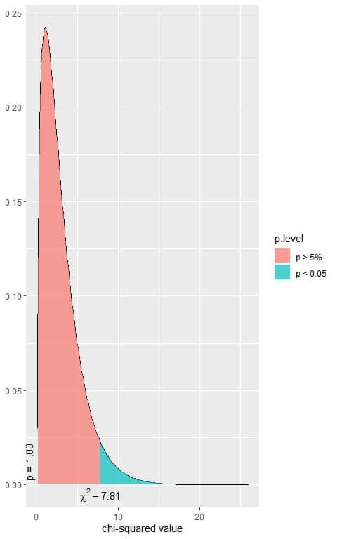 Is that a significant result?
5. The demographic information on every member of a random 2000 sample of the US armed forces showed the following table.
| asian | black | white | Sum |
air force | 11 | 91 | 364 | 466 |
army | 38 | 176 | 586 | 800 |
marine corps | 6 | 39 | 250 | 295 |
navy | 30 | 99 | 310 | 439 |
Sum | 85 | 405 | 1510 | 2000 |
The rows are for the branch of the armed forces: air force, army, marine corps, or navy, and the columns for the race.
All expected values are larger than 5 so the chi-square test can be used.
The χ^2 statistic = 30.051.
The following is the chi-square distribution with 6 df.
 Is that a significant result?
6. Answer key
1. We follow the same steps above to calculate the expected table.
| LEGAL | NOT LEGAL | Sum |
BACHELOR | 110.63781 | 120.36219 | 231 |
GRADUATE | 65.13741 | 70.86259 | 136 |
HIGH SCHOOL | 292.63940 | 318.36060 | 611 |
JUNIOR COLLEGE | 41.18983 | 44.81017 | 86 |
LT HIGH SCHOOL | 93.39555 | 101.60445 | 195 |
Sum | 603.00000 | 656.00000 | 1259 |
We see that all expected values are larger than 5 so the chi-square test can be used.
Then, we follow the above steps to get the chi-square statistic.
The χ^2 statistic = 20.48.
In our 5X2 contingency table, the df = (5-1)X(2-1) = 4.
The following is the chi-square distribution with 4 df.

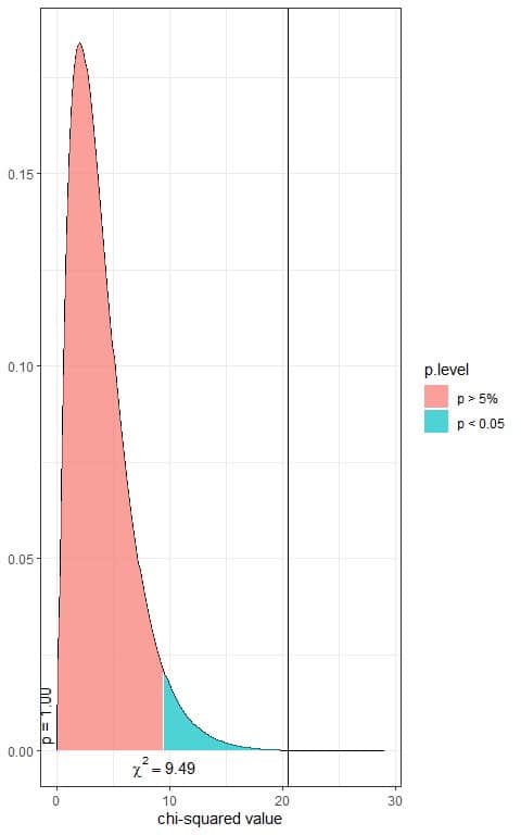
In the first plot, we see that when the χ^2 value = 9.49, the area to the right or the p-value = 0.05.
In our contingency table, the χ^2 value = 20.48 (plotted as a vertical line in the second plot), so the p-value is very much smaller than 0.05.
The p-value < 0.05, so it is a statistically significant result.
We reject the null hypothesis and conclude that there is a significant relationship between the different educational degrees and the response type in the persons surveyed.
This means that the proportions of response type are different across different educational degrees.
2. We follow the same steps above to calculate the expected table.
| Other | Black | White | Sum |
$25000 or more | 714.51932 | 1059.61575 | 5588.8649 | 7363 |
$20000 – 24999 | 124.50473 | 184.63765 | 973.8576 | 1283 |
$15000 – 19999 | 101.69988 | 150.81859 | 795.4815 | 1048 |
$10000 – 14999 | 113.34491 | 168.08790 | 886.5672 | 1168 |
$8000 to 9999 | 32.99424 | 48.92970 | 258.0761 | 340 |
$7000 to 7999 | 18.24387 | 27.05524 | 142.7009 | 188 |
$6000 to 6999 | 20.86400 | 30.94084 | 163.1952 | 215 |
$5000 to 5999 | 22.02851 | 32.66777 | 172.3037 | 227 |
$4000 to 4999 | 21.93146 | 32.52386 | 171.5447 | 226 |
$3000 to 3999 | 26.78356 | 39.71940 | 209.4970 | 276 |
$1000 to 2999 | 38.33154 | 56.84479 | 299.8237 | 395 |
Lt $1000 | 27.75398 | 41.15851 | 217.0875 | 286 |
Sum | 1263.00000 | 1873.00000 | 9879.0000 | 13015 |
We see that all expected values are larger than 5 so the chi-square test can be used.
Then, we follow the above steps to get the chi-square statistic.
The χ^2 statistic = 148.13.
In our 12X3 contingency table, the df = (12-1)X(3-1) = 22.
The following is the chi-square distribution with 22 df.
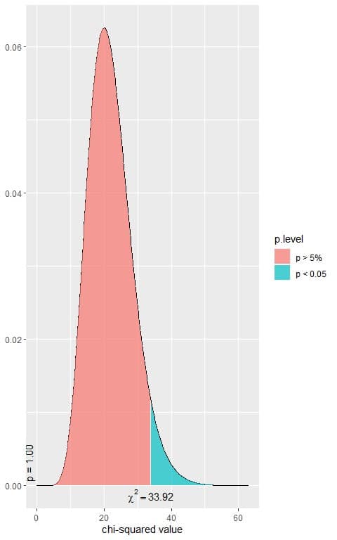
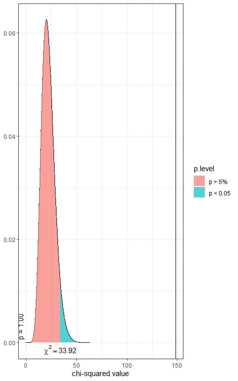
In the first plot, we see that when the χ^2 value = 33.92, the area to the right or the p-value = 0.05.
In our contingency table, the χ^2 value = 148.13 (plotted as a vertical line in the second plot), so the p-value is very much smaller than 0.05.
The p-value < 0.05, so it is a statistically significant result.
We reject the null hypothesis and conclude that there is a significant relationship between race and the reported income in the persons surveyed.
This means that the proportions of incomes are different across different races.
3. We see, from the plot, that when the χ^2 value = 3.84, the area to the right or the p-value = 0.05.
In our contingency table, the χ^2 value = 5.1692, so the p-vale is smaller than 0.05.
The p-value < 0.05, so it is a statistically significant result.
We reject the null hypothesis and conclude that there is a significant relationship between gender and being promoted.
This means that the proportions of promotions are different across the 2 sexes.
4. We see, from the plot, that when the χ^2 value = 7.81, the area to the right or the p-value = 0.05.
In our contingency table, the χ^2 value = 17.534, so the p-vale is smaller than 0.05.
The p-value < 0.05, so it is a statistically significant result.
We reject the null hypothesis and conclude that there is a significant relationship between gender and the branch of the armed forces.
This means that the proportions of branches from the US armed forces are different across the 2 sexes.
5. We see, from the plot, that when the χ^2 value = 12.59, the area to the right or the p-value = 0.05.
In our contingency table, the χ^2 value = 30.051, so the p-value is smaller than 0.05.
The p-value < 0.05, so it is a statistically significant result.
We reject the null hypothesis and conclude that there is a significant relationship between race and the branch of the armed forces.
This means that the proportions of branches are different across the different races.