Column Vector – Explanation & Examples
 A column vector is a matrix with 1 column. Let’s take a look at a formal definition of a column vector.
A column vector is a $ m \times 1 $ matrix consisting of a single column with m elements.
In this article, we will look at what a column vector is, their examples, and matrix operations with column vectors.
What is a Column Vector?
As mentioned earlier, a column vector is a type of matrix with only $ 1 $ column. Column vectors are also known as column matrices. There can be $ 1 $ row, $ 2 $ rows, $ 3 $ rows, or $ n $ rows. But the number of column is always $ 1 $! Below, we show this:
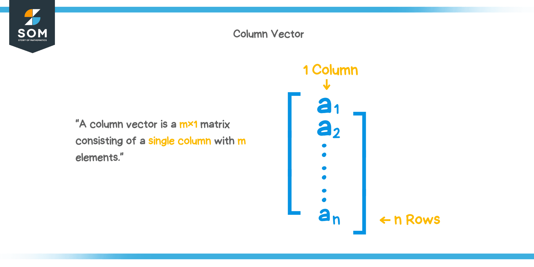
This shows a column vector, $ A $, with $ 1 $ column and $ n $ rows. The first element of the matrix is $ a_1 $, the second element is $ a_2 $, and so on until the last element, $ a_n $. Let us see some column vectors below:
$ \begin{bmatrix} 5 \end {bmatrix} $
This is the simplest column vector with $ 1 $ column and $ 1 $ row. The only element in this matrix is $ 5 $.
$ \begin{bmatrix} { – 3 } \\ { – 5 } \end {bmatrix} $
This is a $ 2 \times 1 $ matrix. There are $ 2 $ rows and $ 1 $ column.
$ \begin{bmatrix} { – 3 } \\ { – 5 } \\ 4 \end {bmatrix} $
This is a $ 3 \times 1 $ matrix. There are $ 3 $ rows and $ 1 $ column. This is a column vector.
Of course, we can have as many rows as we want, but the number of column needs to be $ 1 $. This is what makes a matrix a column vector!
Transpose of Column Vector
Recall that taking the transpose of a matrix means to interchange the rows with columns. The rows become columns and the columns become rows.
What happens when we take the transpose of a column vector?
Since there is only $ 1 $ column, transposing a column vector makes it a row vector! Suppose we have a column vector $ A $:
$ A = \begin{bmatrix} { – 2 } \\ { – 1 } \\ 13 \end {bmatrix} $
If we transpose it, we have a row vector, shown below (let’s call it matrix $ B $):
$ B = \begin{bmatrix} { – 2 } & { – 1 } & 13 \end {bmatrix} $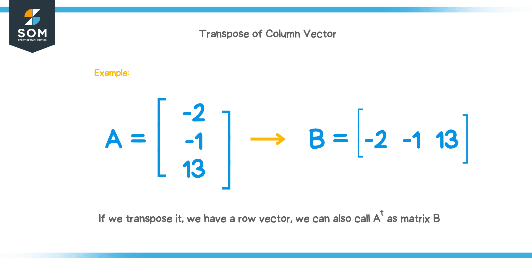
To read more about row vectors, please go here.
How to find a Column Vector
Just like with matrices, we can perform the arithmetic operations on column vectors as well. We will look at addition, subtraction, and scalar multiplication.
Addition
Before adding $ 2 $ column vectors, we have to check whether they are of the same dimensions. If they aren’t, we can’t add them. If they are, we just add the corresponding elements of each column vector. Consider matrices $ A $ and $ B $ shown below:
$ A = \begin{bmatrix} { – 2 } \\ 3 \end {bmatrix} $
$ B = \begin{bmatrix} 8 \\ 4 \end {bmatrix} $
Matrices $ A $ and $ B $ are both $ 2 \times 1 $ matrices. We add the two column vectors by adding the corresponding entries. Shown below:
$ A + B = \begin{bmatrix} { – 2 + 8 } \\ 3 + 4 \end {bmatrix} $
$ A + B = \begin{bmatrix} { 6 } \\ 7 \end {bmatrix} $
Subtraction
Subtraction follows the same rule as addition. We just subtract each corresponding entries. Consider matrices $ C $ and $ D $ shown below:
$ C = \begin{bmatrix} { – 5 } \\ 5 \end {bmatrix} $
$ D = \begin{bmatrix} { – 1 } \\ { – 6 } \end {bmatrix} $
Matrices $ C $ and $ D $ are both $ 2 \times 1 $ matrices. We subtract the two column vectors by subtracting the corresponding entries. Shown below:
$ C – D = \begin{bmatrix} { – 5 – (-1) } \\ 5 – (-6) \end {bmatrix} $
$ C – D = \begin{bmatrix} { -5 + 1 } \\ 5 + 6 \end {bmatrix} $
$ C – D = \begin{bmatrix} { – 4 } \\ 11 \end {bmatrix} $
Scalar Multiplication
When we want to multiply a column vector by a scalar, we simply multiply each element of the column matrix by the scalar. Consider matrix $ A $ shown below:
$ A = \begin{bmatrix} { – 2 } \\ 3 \\ { – 6 } \end {bmatrix} $
If we want to multiply this column matrix by the scalar $ 6 $, we will do so by multiplying each of its entries by $ 6 $. Shown below:
$ 6A = 6 \times \begin{bmatrix} { – 2 } \\ 3 \\ { – 6 } \end {bmatrix} $
$ = \begin{bmatrix} {6 \times – 2 } \\ 6 \times 3 \\ { 6 \times – 6 } \end {bmatrix} $
$ = \begin{bmatrix} { -12 } \\ 18 \\ { -36 } \end {bmatrix} $
Let’s take a look at some examples to clarify our understanding further.
Example 1
Out of the 4 matrices shown below, identify which of them are column vectors.
$ A = \begin{bmatrix} { -2 } \\ 6 \\ { -2 } \end {bmatrix} $
$ B = \begin{bmatrix} { 0 } \\ 0 \\ { 0 } \\ 1 \\ 0 \end {bmatrix} $
$ C = \begin{bmatrix} { -12 } & 6 \end {bmatrix} $
$ D = \begin{bmatrix} { – 43 } \end {bmatrix} $
Solution
- Matrix $ A $ is a $ 3 \times 1 $ matrix. It has $ 3 $ rows and $ 1 $ column. Thus, it is a column vector.
- Matrix $ B $ is s $ 5 \times 1 $ matrix. It has $ 5 $ rows and $ 1 $ column. Most of the entries are zeros, but that doesn’t really matter. Since it has a single column, it is a column vector.
- Matrix $ C $ is a $ 1 \times 2 $ matrix. It has $ 1 $ row and $ 2 $ column. It is not a column vector, rather a row vector.
- Matrix $ D $ is a $ 1 \times 1 $ matrix. It is the simplest form of a matrix. It has $ 1 $ row and $ 1 $ column. It is the simplest column matrix. It is a column vector.
Example 2
What is the transpose of the following column vector?
$ \begin{bmatrix} { – 6 } \\ 0 \\ 9 \\ {-1} \end {bmatrix} $
Solution
Recall that the transpose of a column vector is a row vector. We just write the same entries as a “row” instead of a column. Thus, the transpose is:
$ \begin{bmatrix} { – 6 } & 0 & 9 & { – 1 } \end {bmatrix} $
Example 3
Add matrix $ F $ and $ G $.
$ F = \begin{bmatrix} -3 \\ 0 \\ -2 \end {bmatrix} $
$ G = \begin{bmatrix} 0 \\ -3 \\ 6 \end {bmatrix} $
Solution
Matrix $ F $ and $ G $ are both $ 3 \times 1 $ matrix. They have the same dimension. Thus, they can be added by adding the corresponding elements to each other. Shown below:
$ F + G = \begin{bmatrix} { – 3+ 0 } \\ 0 + -3 \\ -2 + 6 \end {bmatrix} $
$ F + G = \begin{bmatrix} { – 3 } \\ { – 3 } \\ 4 \end {bmatrix} $
Practice Questions
- Find the transpose of:
- $ \begin{pmatrix} a \\ b \\ c \\ e \\ g \end {pmatrix} $
- $ \begin{pmatrix} z \end{pmatrix} $
- Perform the indicated operation for the matrices shown below:
$ A = \begin{pmatrix} 1 \\ { 0 } \\ { – 2 } \\ 8 \end {pmatrix} $$ B = \begin{pmatrix} 3 \\ { 4 } \\ 3 \end {pmatrix} $
$ C = \begin{pmatrix} -9 \\ { 1 } \\ { 1 } \end {pmatrix} $
$ D = \begin{pmatrix} 2 & { 3 } & { – 2 } & 9 \end {pmatrix} $
- $ -3A $
- $ A + D $
- $ B – C $
Answers
- To find the transpose of a column vector, write the column as rows, that’s it!
- $ \begin{pmatrix} a & b & c & e & g \end {pmatrix} $
- $ \begin{pmatrix} z \end{pmatrix} $
Note, the transpose of a $ 1 \times 1 $ matrix is itself!
- Part (a) is scalar multiplication. We multiply each entry of matrix $ A $ by the scalar, $ { – 3 } $.
Part (b) is addition. Since the dimension of matrix $ A $ is not the same as matrix $ D $, we can’t perform the addition.
Part (c) is subtraction. Both matrix $ B $ and $ C $ are $ 3 \times 1 $ matrices. Thus, subtraction can be performed.
All of the answers are shown below:
- $ -3A = { – 3 } \times \begin{pmatrix} 1 \\ { 0 } \\ { – 2 } \\ 8 \end {pmatrix} $
$ = \begin{pmatrix} -3 \times 1 \\ { -3 \times 0 } \\ { -3 \times – 2 } \\ -3 \times 8 \end {pmatrix} $
$ = \begin{pmatrix} -3 \\ 0 \\ 6 \\ -24 \end{pmatrix} $ - Addition not possible!
- $ B – C = \begin{pmatrix} 3 \\ { 4 } \\ 3 \end {pmatrix} – \begin{pmatrix} -9 \\ 1 \\ 1 \end{pmatrix} $
$ B – C = \begin{pmatrix} 3 – – 9 \\ 4 – 1 \\ 3 – 1 \end{pmatrix} $
$ B – C = \begin{pmatrix} 12 \\ 3 \\ 2 \end{pmatrix} $
- $ -3A = { – 3 } \times \begin{pmatrix} 1 \\ { 0 } \\ { – 2 } \\ 8 \end {pmatrix} $