JUMP TO TOPIC
Concavity calculus – Concave Up, Concave Down, and Points of Inflection
 Concavity in Calculus helps us predict the shape and behavior of a graph at critical intervals and points. Knowing about the graph’s concavity will also be helpful when sketching functions with complex graphs.
Concavity calculus highlights the importance of the function’s second derivative in confirming whether its resulting curve concaves upward, downward, or is an inflection point at its critical points.
Our discussion will focus on the following concepts and techniques:
- Identifying concavity and points of inflections given a function’s graph.
- Applying the second derivative test to determine the concavity of a function at different critical points.
- Understanding the relationship between $f(x)$, $f^{\prime}(x)$, and $f^{\prime\prime} (x)$ and how it affects the function’s shape.
Review your derivative rules as well since we’ll have to apply them when finding the expressions of $ f^{\prime}(x)$ and $f^{\prime\prime}(x)$. We’ll assume knowledge of the first and second derivatives throughout the discussion, so make sure to take a quick refresher when you need to.
What is concavity?
Concavity tells us the shape and how a function bends throughout its interval. When given a function’s graph, observe the points where they concave downward or downward. These will tell you the concavity present at the function.
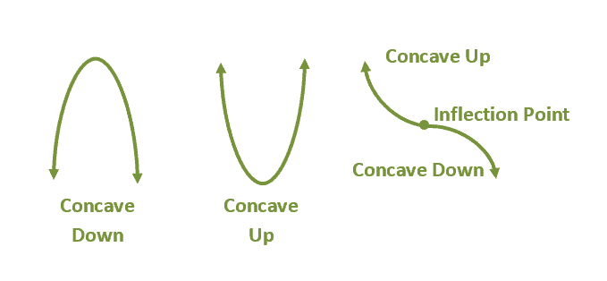
It’s also possible to find points where the curve’s concavity changes. We call these points inflection points. The three examples shown above can guide you in identifying the concavity of a function given its curve as well.

Here’s an example of a graph that exhibits all three concavity types.
- From this, we can see that when a curve is concaving upward, expect a local minimum at the critical point.
- Similarly, at the point where the curve concaves downward, lookout for a local maximum at the critical point.
- Observe how the inflection point is the turning point between these two concavities.
In the next section, we’ll learn how to apply the second derivative test to confirm the concavity of a function given its expression.
How to determine the concavity of a function?
Let’s begin this section by observing these three graphs showing how the curves of $f(x)$, $f^{\prime} (x)$, and $f^{\prime\prime}(x)$ are behaving at the critical numbers, $x=\{0, 1, 2\}$.
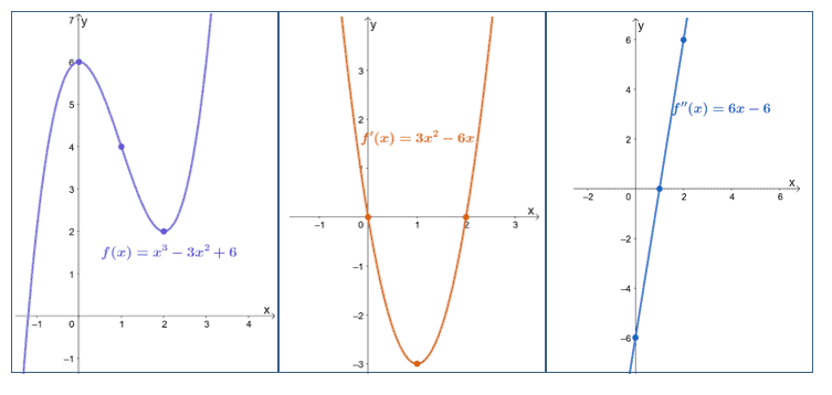
From $f(x)$’s graph, we can see that $x = 0$ is a relative maximum and the curve is concaving upward. The point at $x = 1$ is an inflection point while $x =2$ is a relative minimum. The graph also concaves downward at $x = 2$.
Now, let’s observe $ f^{\prime}(x)$ and $f^{\prime\prime}(x)$’s graphs:
- The sign of $ f^{\prime}(x)$ changes from positive to negative within the interval that contains $x=0$.
- Similarly, $ f^{\prime}(x)$’s signs change from negative to positive within the interval that contains $x=2$.
- When $x = 0$, $f^{\prime\prime}(x)$ is negative while $f^{\prime\prime}(x)$ is positive when $x = 2$.
- Focusing on $x=1$, we can see that $ f^{\prime}(x)$ is equal to 0 and so is $f^{\prime\prime}(x)$.
These observations show us that when the function is concaving downward at a critical point, $x=c$, the second derivative is negative. Similarly, when the function’s curve is concaving upward, $f^{\prime\prime}(x)$ is positive.
Test for concavity
When the function, $f(x)$, is continuous and twice differentiable, we can use its second derivative to confirm concavity.
- When $f^{\prime\prime}(x) >0$, the graph is concaving upward.
- When $f^{\prime\prime}(x) <0$, the graph is concaving downward.
- When $f^{\prime\prime}(x) = 0$, the graph has an inflection point.
What if we can’t differentiate$f(x)$ twice in a row? Use the observations we had about the function’s first derivative instead.
- When $f^{\prime}(x)$’s sign changes from positive to negative, the graph’s curve is concaving downward.
- When $f^{\prime}$’s sign changes from negative to positive, the graph’s curve is concaving upward.
When given a function, find the second derivative of the function right away. Equate the second derivative to zero. Use the solutions to divide the function’s domain into smaller intervals then find a test value to determine the function’s concavity at the intervals.
Let’s say we have $f(x) = x^4 – 4x^2$. To predict its curve’s concavity, we differentiate $f(x)$ twice in a row as shown below.
\begin{aligned}f(x)&=x^4 – 8x^2\\f^{\prime}&= 4x^{3-1} -8(2x^{2-1}),\phantom{x}\color{Teal} \text{Power Rule & Constant Multiple Rule}\\&=4x^3 -16x\\\\ f^{\prime\prime}(x) &=4(3x^{3-1})-16(x^{1 -1}) ,\phantom{x}\color{Teal} \text{Power Rule & Constant Multiple Rule}\\&=12x^2 – 16\end{aligned}
Equate $f^{\prime\prime}(x)$ to 0 so that we can divide the domain of $f(x)$ into smaller intervals.
\begin{aligned}f^{\prime\prime}(x)&=12x^2 – 16\\12x^2-16 &= 0\\12x^2&= 16\\x^2&= \dfrac{4}{3}\\x&=\pm\dfrac{2}{\sqrt{3}}\\&\approx 1.15\end{aligned}
Let’s use the approximate values of $x$ since we just need to find test values that are within the intervals: $\left(-\infty, -\dfrac{2}{\sqrt{3}}\right)$, $\left(-\dfrac{2}{\sqrt{3}},\dfrac{2}{\sqrt{3}}\right)$, and $\left(\dfrac{2}{\sqrt{3}}\right)$.
| Interval | Test Value | Sign of $\boldsymbol{ f^{\prime\prime}(x)}$ | Concavity |
| \begin{aligned}(-\infty, -1.15)\end{aligned} | \begin{aligned} x&= -3\end{aligned} | \begin{aligned} f^{\prime\prime}(-3)&= 12(-3)^2 -16\\&= 92\\&\Rightarrow \color{Teal}\text{Positive}\end{aligned} | Concave upward |
| \begin{aligned}\left(-1.15, 1.15\right)\end{aligned} | \begin{aligned} x&= 1\end{aligned} | \begin{aligned} f^{\prime\prime}(-1)&= 12(-1)^2 -16\\&= -4\\&\Rightarrow \color{Orchid}\text{Negative}\end{aligned} | Concave downward |
| \begin{aligned} (1.15,\infty)\end{aligned} | \begin{aligned} x&= 3\end{aligned} | \begin{aligned} f^{\prime\prime}(3)&= 12(3)^2 -16\\&= 92\\&\Rightarrow \color{Teal}\text{Positive}\end{aligned} | Concave upward |
Our results show that the curve of $f(x)$ is concaving downward at the interval, $\left(-\dfrac{2}{\sqrt{3}},\dfrac{2}{\sqrt{3}}\right)$. Meanwhile, the function’s curve is concaving upward at the intervals, $\left(-\infty, -\dfrac{2}{\sqrt{3}}\right)$ and $\left(\dfrac{2}{\sqrt{3}}\right)$.
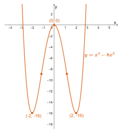
The graph above shows the curve of $f(x)$ and confirms its concavity. We’ve included the inflection points and their values can be confirmed by finding the function’s value at $x = \pm \dfrac{2}{\sqrt{3}}$.
\begin{aligned}f\left(\pm\dfrac{2}{\sqrt{3}} \right )&= \left(\pm\dfrac{2}{\sqrt{3}}\right)^4 -8\left(\pm\dfrac{2}{\sqrt{3}} \right )^2\\&=-\dfrac{80}{9}\\&\Rightarrow \left(-\dfrac{2}{\sqrt{3}}, -\dfrac{80}{9} \right ),\left(\dfrac{2}{\sqrt{3}}, -\dfrac{80}{9} \right )\end{aligned}
This means that $f(x)$ has inflection points at $\left(-\dfrac{2}{\sqrt{3}}, -\dfrac{80}{9} \right )$ and $\left(\dfrac{2}{\sqrt{3}}, -\dfrac{80}{9} \right )$.
How to compare concave up vs concave down?
Let’s summarize what we’ve just learned throughout the discussion by comparing the curves that concave upward or downward.
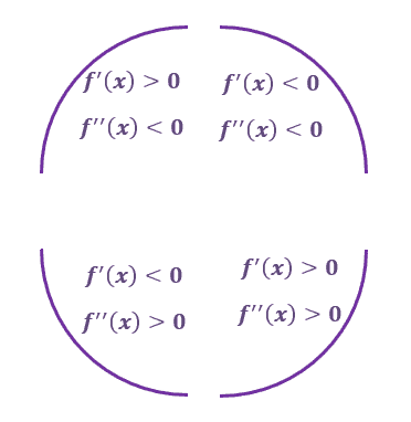
The four curves below will guide you in knowing the curve’s behavior given its first and second derivatives at the point. Let’s use these to highlight the difference between a curve that concaves upward or downward.
Concave up
The upper half breaks down the behavior of $ f^{\prime}(x)$ and $ f^{\prime\prime}(x)$ when the curve is concaving upwards.
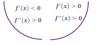
This shows that the function’s second derivative is positive when the curve is concaving upward. When the curve is concaving upward, the function is decreasing then increasing. This means that $\boldsymbol{f^{\prime}(x)}$ changes from positive to negative.
Concave down
The upper half tells us that when the curve is concaving downward, the second derivative of the function at that point is negative.
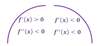
The first derivative of the function is positive from the left and negative from the right of the critical point. This means that the curve concaving downward is increasing from the left and decreasing from the right.
Inflection point
We can’t discuss concavity without summarizing what we know about inflection points.
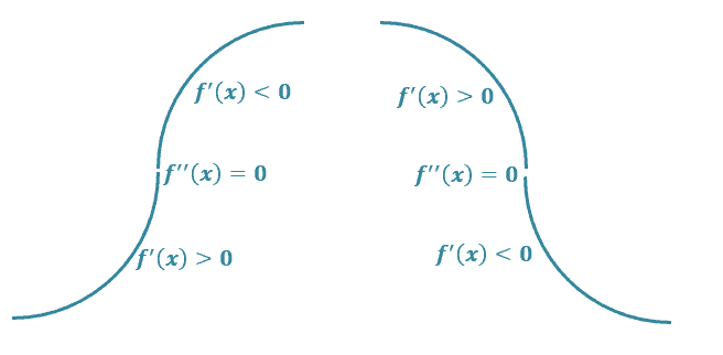
We can’t discuss concavity without summarizing what we know about inflection points. Inflection points are located at values of $\boldsymbol{x}$ the curve changes concavity. Keep in mind that at this point, $\boldsymbol{f^{\prime\prime}(x)}$ is equal to zero.
This section summarizes what we’ve just learned about concavities. Review the example we’ve shown you in our discussion too. Once you’re ready, dive right into these sample problems we’ve prepared just for you!
Example 1
Given $f(x) = x^3−24x^2+24$, find the open intervals where $f(x)$’s curve is concaving upward or downward.
Solution
We begin by differentiating $f(x)$ twice in row to determine the expression for $f^{\prime \prime}$.
\begin{aligned}f(x)&=x^3- 12x^2 +24\\f^{\prime}(x)&=\dfrac{d}{dx}x^3 -\dfrac{d}{dx}12x^2+ \dfrac{d}{dx}24, \phantom{x}\color{Teal}\text{Sum & Difference Rules}\\&=\dfrac{d}{dx}x^3 -\dfrac{d}{dx}12x^2+ 0, \phantom{x}\color{Teal}\text{Constant Rule}\\&= 3x^{3-1} – 12(2x^{2-1}),\phantom{x}{\color{Teal} \text{Constant Multiple & Power Rules}}\\&= 3x^2-24x\\\\f^{\prime\prime}(x) &= 3(2x^{2 -1})-24(x^{1- 1}),\phantom{x}{\color{Teal} \text{Constant Multiple & Power Rules}}\\&=6x – 24\end{aligned}
Now that we have $f^{\prime \prime}(x)$, equate the expression to $0$ then find $x$. Use the values of $x$ to divide the domain of $f(x)$ into smaller intervals.
\begin{aligned}f^{\prime\prime}(x) &=0\\6x – 24&= 0\\6x &= 24\\x &=4\end{aligned}
Observe the signs of $f^{\prime\prime}(x)$ for the intervals, $(-\infty, 4)$ and $(4, \infty)$. When $f^{\prime \prime}(x)$ is negative, $f(x)$ is concaving downward. Similarly, when $f^{\prime \prime}(x)$ is positive, $f(x)$ is concaving upward.
| Interval | Test Value | Sign of $\boldsymbol{ f^{\prime\prime}(x)}$ | Concavity |
| \begin{aligned}(-\infty, 4)\end{aligned} | \begin{aligned} x&= -4\end{aligned} | \begin{aligned} f^{\prime\prime}(1)&= 6(1) -24 \\&=-18\\&\Rightarrow \color{Orchid}\text{Negative}\end{aligned} | Concave downward |
| \begin{aligned}(4,\infty)\end{aligned} | \begin{aligned} x&= 4\end{aligned} | \begin{aligned} f^{\prime\prime}(5)&= 6(5) – 24\\&=6\\&\Rightarrow \color{Teal}\text{Positive}\end{aligned} | Concave upward |
From the table, we can see that $f(x)$ is concaving downward within the interval of $(-\infty, 4)$. The function is concaving upward within the interval of $(4, \infty)$.
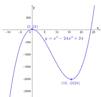
Here’s the graph of $f(x)$ and this confirms the concavity within the two intervals, $(-\infty, 4)$ and $(4, \infty)$.
Example 2
Given $f(x) = 3x^2 – \dfrac{1}{x^2}$, find its points of inflection. Discuss the concavity of the function’s graph as well. Form the acquired information, roughly sketch the graph of $f(x)$.
Solution
Recall that $\dfrac{1}{x^2} = x^{-2}$, so we can rewrite $f(x)$ first to differentiate it much faster. Find $f^{\prime \prime}(x)$ by differentiating $f(x)$ twice in a row as shown below.
\begin{aligned}f(x) &= 3x^2 – \dfrac{1}{x^2}\\&= 3x^2 – x^{-2}\\f^{\prime}(x) &= 3(2x^{2 -1}) – (-2)x^{-2 -1},\phantom{x}\color{Teal}\text{Constant Multiple & Power Rules}\\&= 6x + 2x^{-3}\\f^{\prime \prime}(x)&= 6(x^{1-1})+2(-3x^{-3 -1}),\phantom{x}\color{Teal}\text{Constant Multiple & Power Rules}\\&=6x^0 – 6x^{-4}\\&= 6 – \dfrac{6}{x^4}\end{aligned}
Equate $f^{\prime\prime}(x)$ to zero then divide the domain of $f(x) = 3x^2 – \dfrac{1}{x^2}$ into smaller intervals.
\begin{aligned}f^{\prime \prime}(x)&=0\\6 – \dfrac{6}{x^4}&= 0\\\dfrac{1}{x^4} &= 1\\x&= \pm 1\end{aligned}
The domain of $f(x)$ is $(-\infty, 0) \cup (0, \infty)$, so we can divide this into smaller intervals to account for $x = \pm 1$. Assign test values that are within the following intervals: $\{(-\infty, -1), (-1, 0), (0, 1), (1, \infty)\}$.
| Interval | Test Value | Sign of $\boldsymbol{ f^{\prime\prime}(x)}$ | Concavity |
| \begin{aligned}(-\infty, -1)\end{aligned} | \begin{aligned} x&= -2\end{aligned} | \begin{aligned} f^{\prime\prime}(-2)&= 6 – \dfrac{6}{(-2)^4}\\&=\dfrac{45}{8}\\&\Rightarrow \color{Teal}\text{Positive}\end{aligned} | Concave upward |
| \begin{aligned}(-1,0)\end{aligned} | \begin{aligned} x&= -\dfrac{1}{2}\end{aligned} | \begin{aligned} f^{\prime\prime}\left(-\dfrac{1}{2} \right )&= 6 – \dfrac{6}{\left(-\dfrac{1}{2} \right )^4}\\&=-90\\&\Rightarrow \color{Orchid}\text{Negative}\end{aligned} | Concave downward |
| \begin{aligned}(0, 1)\end{aligned} | \begin{aligned} x&= \dfrac{1}{2}\end{aligned} | \begin{aligned} f^{\prime\prime}\left(\dfrac{1}{2} \right )&= 6 – \dfrac{6}{\left(\dfrac{1}{2} \right )^4}\\&=-90\\&\Rightarrow \color{Orchid}\text{Negative}\end{aligned} | Concave downward |
| \begin{aligned}(1,\infty)\end{aligned} | \begin{aligned} x&= 2\end{aligned} | \begin{aligned} f^{\prime\prime}(2)&= 6 – \dfrac{6}{(2)^4}\\&=\dfrac{45}{8}\\&\Rightarrow \color{Teal}\text{Positive}\end{aligned} | Concave upward |
We can see that $f(x)$ concaves downward for the intervals, $(-1,0)$ and $(0, 1)$. Meanwhile, the curve concaves upwards for the intervals, $(-\infty, -1)$ and $(1, \infty)$.
Moving on to $f(x)$’s points of inflection, let’s go back to the values of $x$ that return $f^{\prime \prime}(x)$ to zero. These are, in fact, the $x$-coordinates of the function’s point of inflections. Substitute $x= \pm 1$ into $f(x)$ to find the $y$-coordinates of $f(x)$’s points of inflection.
\begin{aligned}f(\pm 1) &=3(\pm 1)^2 – \dfrac{1}{(\pm 1)^2}\\&= 3 -1\\&=2\\&\Rightarrow (-1,2), (1, 2) \end{aligned}
Hence, $f(x)$ has points of inflection at $(-1, 2)$ and $(1, 2)$. Use the concavity, points of inflection, and asymptotes of $f(x)$ to roughly sketch its graph.
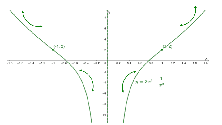
This graph highlights where the concavities are located for this function. Don’t worry, we’ll be able to have a better approximation of the graph once we learn about curve sketching using derivatives. For now, it’s a sneak peek at one of the many applications of concavity in calculus.
Practice Questions
1. Given the functions shown below, find the open intervals where each function’s curve is concaving upward or downward.
a. $f(x) = x^3 – 12x + 18$
b. $g(x) = \dfrac{1}{4}x^4 – \dfrac{1}{3}x^3 + \dfrac{1}{2}x^2$
c. $h(x) =x^5 – 270x^2 + 1$
2. Given the functions shown below, find the open intervals where each function’s curve is concaving upward or downward.
a. $f(x) = \dfrac{x}{x+1}$
b. $g(x) = x\sqrt{x^2 -1}$
c. $h(x) =4x^2 – \dfrac{1}{x}$
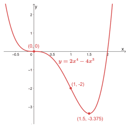
3. Given $f(x) = 2x^4 – 4x^3$, find its points of inflection. Discuss the concavity of the function’s graph as well. Form the acquired information, roughly sketch the graph of $f(x)$.
Answer Key
1.
a. Concave downward: $(-\infty, 0)$; Concave upward: $(0, \infty)$
b. Concave upward throughout the domain – $(-\infty, \infty)$.
c. Concave downward: $(-\infty, 3)$; Concave upward: $(3, \infty)$
2.
a. Concave downward: $(-\infty, -1)$; Concave upward: $(-1, \infty)$
b. Concave downward: $\left(-\infty, -\sqrt{\dfrac{3}{2}}\right)$ and $\left(1,\sqrt{\dfrac{3}{2}}\right)$; Concave upward: $\left(-\sqrt{\dfrac{3}{2}}, -1\right)$ and $\left(\sqrt{\dfrac{3}{2}}, \infty\right)$
c. Concave downward: $\left(0, \dfrac{\sqrt[3]{2}}{2}\right)$; Concave upward: $\left(-\infty, 0\right)$ and $\left(\dfrac{\sqrt[3]{2}}{2}, \infty\right)$
3.
Concavity: Concave downward: $(0, 1)$; Concave upward: $(-\infty, 0)$ and $(1, \infty)$
Points of Inflection: $(0,0)$ and $(1, -2)$
Graph:
Images/mathematical drawings are created with GeoGebra.