Correlation Coefficient – Explanation and Examples

The correlation coefficient of a set of data is a number between $-1$ and $1$ that shows how random the data is.

A number closer to $0$ indicates randomness. A number closer to $1$ indicates a positive correlation, while a number closer to $-1$ indicates a negative correlation.

Correlation coefficients are important for any kind of statistical analysis. The higher the absolute value of the correlation coefficient, the stronger the association between two variables.

This section covers:

• What is a Correlation Coefficient?
• Correlation Coefficient Definition
• How to find Correlation Coefficient
• Method 1 for Calculating the Correlation Coefficient
• Method 2 for Calculating the Correlation Coefficient
• Relationship to Linear Regressions
• History of Correlation Coefficient
• Interpreting the Correlation Coefficient

What Is a Correlation Coefficient?

A correlation coefficient is a number that shows how strongly two variables are associated. This number can be any value between $-1$ and $1$. The closer the absolute value of the coefficient is to 1, the stronger the association between the two variables.

Specifically, values closer to $1$ indicate a strong positive association, while values closer to $-1$ show a strong negative association. That is, when the value is closer to $1$, the value of the dependent variable will increase as the independent variable increases. The opposite is true when the correlation coefficient is closer to $-1$.

When the correlation coefficient is closer to $0$, it indicates a lack of association between the two variables.

A correlation coefficient greater than $0.8$ or less than $-0.8$ is generally considered significant.

Correlation Coefficient Definition

A correlation coefficient is a number between $1$ and $-1$ that shows how associated two variables are. Usually, this number is denoted as $r$.

Random data will have values closer to $0$, proportional data will have values closer to $1$, and inversely proportional data will have values closer to $-1$.

Numerically, the correlation coefficient is equal to the covariance of the $x$ and $y$ values divided by the product of the standard deviations of $x$ and $y$.

This is:

$\frac{cov(x, y)}{\sigma_x\sigma_y}$.

Covariance

Covariance is a way of measuring how two variables relate to each other. Suppose the larger values of one variable correspond to lower values of the other, then the covariance is negative. If the opposite is true, that larger values of one variable correspond to higher values of the other, the covariance is positive.

Just like the correlation coefficient, the sign of covariance indicates the type of relationship between two variables.

Covariance, however, is not normalized. This means that it is difficult to interpret its magnitude without a lot of contexts.

The correlation coefficient is essentially covariance normalized. That is, it makes it easy to determine the direction and strength of a relationship between two variables. The covariance only indicates the direction.

How to Find Correlation Coefficient

The correlation coefficient is meaningful for bivariate quantitative data. That is when the data consists of two numerical values. For example, height and shoe size or temperature and humidity are bivariate quantitative data.

The correlation coefficient shows whether or not the data have a linear relationship.

Calculating this number by hand is certainly possible, but it takes a significant amount of time, especially as the number of data points increases.

For this reason, it is much more common to use a calculator to find the correlation coefficient. Most have a function that will find this number for a given set of data. Alternatively, even a simple calculator can help to find the sums and square roots necessary for calculating a correlation coefficient the long way.

There are two main methods for finding the correlation coefficient.

This first method uses the numerical definition of covariance of $x$ and $y$ divided by the product of the standard deviations of $x$ and $y$.

Method 1 for Calculating the Correlation Coefficient

To calculate $r$ for bivariate data with independent variable $x$ and dependent variable $y$ by hand using method 1:

1. Calculate the mean of all the $x$ values, $\bar{x}$.
   If there are $n$ data points, the mean is $\bar{x}=\frac{\sum\limits_{k=1}^n x_k}{n}$. That is the sum of all the $x$ terms divided by the total number of terms.
2. Calculate the mean of all the $y$ values, $\bar{y}$.
   If there are $n$ data points, the mean is $\bar{y}=\frac{\sum\limits_{k=1}^n y_k}{n}$. The sum of all the $y$ terms is divided by the total number of terms.
3. Calculate the standard deviation of all the $x$ terms, $s_x$.
   The standard deviation is $s_x$=$\sqrt{\frac{\sum\limits_{k=1}^n (x_k-\bar{x})^2}{n-1}}$. This is a complicated-looking formula, but it simply finds how much the typical data point deviates from the mean.
4. Calculate the standard deviation of all the $y$ terms, $s_y$.
   The standard deviation is $s_y$=$\sqrt{\frac{\sum\limits_{k=1}^n (y_k-\bar{y})^2}{n-1}}$. Again, this is a complicated-looking formula, but remember it just finds how much the typical data point deviates from the mean.
5. Next, use the means to find the covariance of $x$ and $y$. The covariance is equal to $\frac{\sum\limits_{k=1}^n (x_k-\bar{x})(y_k-\bar{y})}{n}$. That is, find the difference between each $x$ value and the mean of $x$ from step $1$. Then multiply that by the difference between the corresponding $y$ value and the mean $y$ from step $2$. Add up all of these products, then divide by $n$, the number of terms.
6. Finally, divide the covariance by the product of the standard deviation of $x$ and the standard deviation of $y$ found in steps $3$ and $4$.

Put another way, $r=$$\frac{\sum\limits_{k=1}^n (x_k-\bar{x})(y_k-\bar{y})}{\sqrt{(\sum\limits_{k=1}^n (x_k-\bar{x})^2)(\sum\limits_{k=1}^n (y_k-\bar{y})^2)}}$.

Method 2 for Calculating the Correlation Coefficient

Using this same equation as above, it is possible to derive another formula for $r$ as:

$\frac{n\sum\limits_{k=1}^n x_k y_k-\sum\limits_{k=1}^n x_k \sum\limits_{k=1}^n y_k }{\sqrt{(n\sum\limits_{k=1}^n x^2 – (\sum\limits_{k=1}^n x)^2)(n\sum\limits_{k=1}^n y^2 – (\sum\limits_{k=1}^n y)^2)}}$.

This equation may look complicated, but it is easier to work with because the necessary sums are simple to find. This formula is used for the second method.

This second method uses the formula above, which is derived from the definitional formula:

1. Find the sum of all of the $x$ values. Additionally, find the square of this number.
2. Then, find the sum of all the squared $x$ values.
3. Next, find the sum of all of the $y$ values. Like step 1, find the square of this number too.
4. After that, find the sum of all of the squared $y$ values.
5. Then, find the sum of the products of each $x$ value, and its corresponding $y$. This is $\sum\limits_{k=1}^n x_ky_k$.
6. Finally, plug all of these values into the formula above and simplify.

Again, despite these formulae looking complicated, they are not too difficult to use. In this case, it helps to make a table of $x$ values, $x^2$ values, $y$ values, $y^2$ values, and $xy$ values. It is easy to move across a row to find the products ($x^2, y^2,$ and $xy$) and move down the columns to find sums.

Linear Regressions

Correlation coefficients are related to linear regressions. These are sometimes called “lines of best fit.” That is, they are a line that best approximates the data.

The correlation coefficient shows how well the regression line fits the data. A larger absolute value of the correlation coefficient indicates a better fit.

In fact, the correlation coefficient for data that perfectly fits the line of best fit will be $1$ or $-1$ (depending on whether the line has a positive or negative slope). A large sample of truly random data, on the other hand, will have a value very close to $0$.

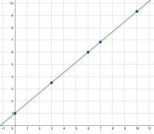
These data points all lie on the line $y=\frac{5}{6}x+1$. One could go through and calculate the correlation coefficient by hand using either of the two methods shown above.

This process, however, would be unnecessary. The correlation coefficient for this data set is $1$ because the data lie exactly on a positive line.

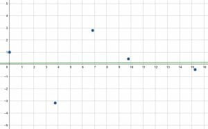
The data above are relatively random points. There is no clear pattern.

The line of best fit shown is almost exactly horizontal. This means there is essentially no relationship between the $x$ and $y$ values. Trying to use this data to predict a future value would be meaningless.

In this case, the correlation coefficient for the data will be very close to $0$.

Note that in some cases, a linear model may not be a good model for the data. In this case, the correlation coefficient may still have a low absolute value. But, modeling it with a cubic, quadratic, or exponential function may more accurately represent the data. It may also make more accurate predictions about unsampled values.

Quadratic Example

The following points lie on the quadratic curve $y=x^2$.

$(-4, 16), (-3, 9), (-2, 4), (-1, 1), (0, 0), (1, 1), (2, 4), (3, 9), (4, 16)$

The line of best fit for this data has the formula $y=0+\frac{2}{3}$.

This relationship has a slope of $0$! That is, it is perfectly horizontal. Therefore, its correlation coefficient is also $0$.

But that doesn’t mean that these points are unrelated! There is just not a good linear model of this data.

History of Correlation Coefficient

The correlation coefficient is also known as the Pearson correlation coefficient. It was named after the famous English statistician Karl Pearson. However, it was not discovered by him.

The naming of the Pearson correlation coefficient after Karl Pearson is a famous example of Stigler’s law of eponymy. This rule states that scientific and mathematical discoveries are never named after the people who actually discovered them. Think, for example, of the Pythagorean Theorem, which was known long before Pythagoras.

In this case, Pearson heard about the concept from the mathematician Francis Galton. Even before Galton, however, a formula for the correlation coefficient came from Auguste Bravais in the 1840s.

Pearson became associated with the idea, however, because he helped develop and promote other statistical concepts. In fact, he is considered one of the main innovators in a modern statistical study.

There are other correlation coefficients. That is, there are other ways to measure how well data conforms to a given line. The Pearson correlation coefficient, however, is the most famous. If someone just says “correlation coefficient,” they almost always mean the Pearson correlation coefficient.

Interpreting Correlation Coefficient

The correlation coefficient is most often used in context with a given equation for linear regression.

Recall that the linear regression or the “line of best fit” is a line that approximates data.

Not all data can be well-modeled by a line. Some data actually follow a curve, as in the quadratic example above. Other times, a lack of sample points makes it difficult to draw accurate conclusions. In this case, one abnormal result can skew an entire data set.

A correlation coefficient with a high absolute value will be closer to $1$ or $-1$. In either case, it indicates that the given line closely approximates the data.

The great thing about this is that a statistician has more evidence to make a claim about an association between the two variables. He can also use the linear model to make predictions about unsampled values, especially larger values.

Examples

This section covers common problems using properties of equality and their step-by-step solutions.

Example 1

Find the standard deviation for $x$ and $y$ in the given data set. Then, interpret the results.

$(0, 3), (3, 6), (6, 7), (7, 10), (10, 9).$

Solution

This problem can be separated into two parts. First, solve for the standard deviation of $x$. Then, solve for the standard deviation of $y$.

Standard Deviation of $x$

Now, it is required to find the standard deviation of the $x$ values, $s_x$. The formula for this is:

$s_x = \sqrt{\frac{\sum \limits_{k=1}^n (x_k-\bar{x})^2}{n-1}}$

Note that this requires first finding the difference between each of the $x$ terms and $\bar{x}$.

In this case, $\bar{x} = \frac{0+3+6+7+10}{5} = \frac{26}{5}$

Next, find the difference between the sampled value and the mean. Then, square this difference.

For each of the sample values, this is:

$(0-\frac{26}{5})^2 = \frac{ 676 }{25}$.

$(3-\frac{26}{5})^2 = \frac{ 121 }{25}$.

$(6-\frac{26}{5})^2 = \frac{ 16 }{25}$.

$(7-\frac{26}{5})^2 = \frac{ 81 }{25}$.

$(10-\frac{26}{5})^2 = \frac{ 576 }{25}$.

Now, recall $s_x$=$\sqrt{\frac{\sum\limits_{k=1}^n (x_k-\bar{x})^2}{n-1}}$. In this case, that is:

$s_x$=$\sqrt{\frac{\frac { 676 }{25} + \frac{121}{25} + \frac{16}{25} + \frac{81}{25} + \frac{576}{25}}{4}}$.

This simplifies to $\sqrt{ \frac{ 147 }{10}}$, which is approximately equal to $3.83$.

Standard Deviation of $y$

Similarly, it is required to find the standard deviation of the $y$ values, $s_y$. That requires finding the difference between each of the $y$ terms and $\bar{y}$.

In this case, $\bar{y}=\frac{3+6+7+10+9}{5} = \frac{35}{5} = 7$

Now, find the difference between each $y$ value and $7$. These will need to then be squared.

$3-7=-4$ and $(-4)^2=16$

$6-7=-1$ and $(-1)^2=1$

$7-7=0$ and $0^2=0$

$10-7=3$ and $3^2=9$

$9-7=2$ and $2^2=4$.

Now, recall $s_y=$$\sqrt{\frac{\sum\limits_{k=1}^n (y_k-\bar{y})^2}{n-1}}$. In this case, that is:

$\sqrt{\frac{16+1+0+9+2}{3}} = \sqrt{\frac{28}{3}}$.

which is approximately equal to $9.33$.

Thus, the standard deviation of $x$ is about $3.83$, and the standard deviation of $y$ is about $9.33$.

In context, this means that the $x$ values tend to be closer to the mean than the $y$ values. That is, there is more variance in the $x$ values than in the $y$ values.

Example 2

Find the covariance for the data set given. Then, interpret the results.

$(1, 3), (-1, -2), (2, 2), (0, 0)$

Solution

The covariance is equal to the sum of the product of the difference between $x$ values and the mean of $x$. And the $y$ values and the mean of $y$ divided by $n$.

Mathematically, the formula for covariance is:

$\frac{\sum \limits_{k=1}^n (x_k-\bar{x})(y_k-\bar{y})}{n}$.

Therefore, first find $\bar{x}$ and $\bar{y}$. These are the means, so they are equal to the sum of the terms divided by the number of terms.

$\bar{x} = \frac{1-1+2+0}{4} = \frac{1}{2}$.

$\bar{y}= \frac{3-2+2+0}{4} = \frac{3}{4}$.

Next, find the difference between each $x$ value and the mean.

$1-\frac{1}{2} = \frac{1}{2}$

$-1-\frac{1}{2} = -\frac{3}{2}$

$2-\frac{1}{2} = \frac{3}{2}$

$0-\frac{1}{2} = -\frac{1}{2}$.

Similarly, find the difference between each $y$ value and the mean.

$3-\frac{3}{4} = \frac{9}{4}$

$-2-\frac{3}{4} = -\frac{11}{4}$

$2-\frac{3}{4} = \frac{5}{4}$

$0-\frac{3}{4} = -\frac{3}{4}$

Next, multiply corresponding differences together and add them up.

$(\frac{1}{2})(\frac{9}{4}) + (-\frac{3}{2})(-\frac{11}{4}) + (\frac{3}{2})(\frac{5}{4}) + (-\frac{1}{2})(-\frac{3}{4}) = \frac{9}{8}+\frac{33}{8} + \frac{15}{8}+\frac{3}{8} = \frac{60}{8} = \frac{15}{2}$.

Therefore, the covariance for this data set is $\frac{15}{2}$. Since this is positive, there is a positive correlation between the two variables. Here, however, since the magnitude is not normalized, it is difficult to tell if this indicates a strong relationship or not.

Example 3

Find the correlation coefficient for this set of data.

$(-2, 3), (-1, 2), (0, 0), (1, 0)$

Solution

There are a few ways to do this problem. First, note that in the second version of the formula for the correlation coefficient, $\frac{n\sum\limits_{k=1}^n x_k y_k-\sum\limits_{k=1}^n x_k \sum\limits_{k=1}^n y_k }{\sqrt{(n\sum\limits_{k=1}^n x^2 – (\sum\limits_{k=1}^n x)^2)(n\sum\limits_{k=1}^n y^2 – (\sum\limits_{k=1}^n y)^2)}}$, only uses $x$, $x^2$, $y$, $y^2$, and $xy$.

The values of $x$ are $-2, -1, 0,$ and $1$. Their sum is $-2$.

From the data, the values of $y$ are $3, 2, 0, 0$. Their sum is $5$.

Multiplying each $x$ by each corresponding $y$ gives $-6, -2, 0, 0$. The sum of these values is $-8$.

Next, square the values of $x$ and $y$. This is $4, 1, 0, 1$ and $9, 4, 0, 0$ respectively. Their sums are $6$ and $13$.

Note also that there are $4$ data points, so $n=4$.

Finally, plug these values into the given formula. It yields:

$r=\frac{4\times-8-(-2)(5)}{\sqrt{(4\times6-(-2)^2)(4\times13-5^2)}}$

This simplifies to:

$r=\frac{-32+10}{\sqrt{(24-4)(52-25)}}$

$r=\frac{-22}{\sqrt{(20)(27)}}$.

Further simplification gives:

$r=\frac{-22}{6\sqrt{(5)(3)}} = \frac{-11}{3\sqrt{15}}$.

Using a calculator approximates this number to $-0.95$.

Example 4

A marine biologist tries to find a relationship between ocean temperature and the presence of a certain type of algae. After taking his samples, he calculates a correlation coefficient for the data.

The data has a correlation coefficient of 0.75. What does this mean in context?

Solution

The correlation coefficient for the scientist’s model is positive, but it is less than $0.8$.

In context, this means that there was generally more algae as the temperature of the water increased. Since the absolute value of the correlation coefficient is less than $0.8$, however, the association was not that strong.

The scientist might be able to make a claim about the positive association based on this data. He probably should not use this model to make predictions about the number of algae present for a certain water temperature.

Example 5

A meteorologist tracks the max temperature and max humidity for eight days. She gets the following results:

$(79, 0.81), (83, 0.53), (82, 0.52), (80, 0.59), (80, 0.60), (83, 0.66), (85, 0.73), (86, 0.74)$

She measured the temperature ($x$) in degrees Fahrenheit and the humidity ($y$) as a percentage. Then, she changed the percentage to a decimal when recording the data.

Use a calculator to find the correlation coefficient. Then, interpret the correlation coefficient in context.

Solution

This problem says explicitly to use a calculator. Most of the time, it is more efficient to use a calculator for these types of problems because of the number and complexity of the steps involved.

Using a calculator, the sum of the $x$ values is $658$, and the sum of $y$ values is $5.2$.

Squaring these values gives $432,964$ and $27.04$, respectively.

Adding up the squares of the $x$ values gives $54,164$. Similarly, the sum of the squares of the $y$ values is $3.4532$.

Adding up the product of corresponding $x$ and $y$ values gives $427.95$ while the product of the sum of $x$ with the sum of $y$ is $3421.6$.

Plugging these values into the equation $\frac{n\sum \limits_{k=1}^n x_k y_k-\sum\limits_{k=1}^n x_k \sum \limits_{k=1}^n y_k }{\sqrt{(n\sum \limits_{k=1}^n x^2 – (\sum \limits_{k=1}^n x)^2)(n\sum\limits_{k=1}^n y^2 – (\sum \limits_{k=1}^n y)^2)}}$ yields:

$\frac{8(427.95)-3421.6}{\sqrt{(8(54,164)-432,964)(8(3.4532)-27.04)}}$

This simplifies to:

$\frac{2}{\sqrt{(348)(0.5856)}}$

$\frac{2}{\sqrt{203.788}}$.

which is approximately equal to $0.14$.

This value is very close to $0$, so there is little association between the variables based on the sample.

Practice Problems

1. Explain why what will happen if one tries to find the correlation coefficient for a sample of only two points.
2. Find the covariance for the data set $(-3, 4), (-1, 5), (0, 6), (1, 5), (3, 10)$.
3. Find the correlation coefficient for the data set $(10, 11), (15, 12), (30, 17), (35, 20), (40, 22)$. It may be more efficient to use a calculator to help.
4. A researcher records the amount of electric used by a home and the home energy bill for $40$ homes in different cities. She finds a correlation coefficient of $0.98$. She used electricity consumption as her $x$ value and energy bill as her $y$ value. What does her data suggest?
5. A psychologist records the amount of time people spend working out every day and the amount of time they spend watching television. He records his data in hours and uses exercise time as the $x$ variable. He gets the following data: $(1, 1), (0, 3), (2, 0), (1, 2), (2, 2), (0, 4), (1, 0), (3, 0)$.
   Find the correlation coefficient for the data and interpret it in context.

Answer Key

1. First of all, note that a sample with only two points will have a line that connects the two points perfectly. Therefore, its correlation coefficient should be exactly $-1$ or $1$ or $0$. It will be $-1$ when the line has a negative slope and $1$ when it has a positive slope. If the line is horizontal, the coefficient will be $0$.
2. $\frac{17}{5}$
3. Approximately $0.99$.
4. Her data suggests that there is a strong positive relationship between the amount of energy used and the energy bill. This makes sense since most people are charged based on actual or estimated energy consumption.
5. The correlation coefficient is $-0.73$. This suggests there is a moderate negative relationship between the two variables. That is, it suggests some decrease in hours watching television when time is spent exercising. Since the absolute value is below $0.8$, however, generalizations and predictions should not be made using this data.

Images/mathematical drawings are created with GeoGebra.