JUMP TO TOPIC
Cumulative Frequency – Explanation & Examples
 The definition of cumulative frequency is:
“The cumulative frequency is the frequency of data points that lie up to a certain value in your data.”
In this topic, we will discuss the cumulative frequency from the following aspects:
- What is the cumulative frequency in statistics?
- How to find cumulative frequency?
- Cumulative frequency formula.
- Practical questions.
- Answers.
What is the cumulative frequency in statistics?
The cumulative frequency is the frequency of data points that lie up to a certain value in your data. Cumulative frequency is used to determine the number of data points that lie above (or below) a certain value in a data set.
The cumulative frequency of a certain data point is the sum of all previous frequencies up to that data point in a frequency table.
The last cumulative frequency value will always be equal to the total number of data points. The data points can be categorical or numeric data.
– Example 1 of categorical data
The following are the smoking habits of 10 participants from a certain survey. Each individual chooses his smoking habit as “Never smoker”, “Current or former < 1y”, for current or former smokers who quit smoking for less than 1 year, or “Former >= 1y” for former smokers who quit smoking for more than or equal to 1 year.
participant | Smoking habit |
1 | Never smoker |
2 | Never smoker |
3 | Current or former < 1y |
4 | Never smoker |
5 | Current or former < 1y |
6 | Never smoker |
7 | Never smoker |
8 | Former >= 1y |
9 | Former >= 1y |
10 | Former >= 1y |
We can list the occurrences of different smoking habits in the following frequency table.
Smoking habit | frequency |
Never smoker | 5 |
Current or former < 1y | 2 |
Former >= 1y | 3 |
We see that the most frequent smoking habit is “Never smoker” with 5 occurrences and the least frequent smoking habit is “Current or former < 1y” smoking habit with only 2 occurrences.
We can add a third column for the cumulative frequency.
Smoking habit | frequency | cumulative frequency |
Never smoker | 5 | 5 |
Current or former < 1y | 2 | 7 |
Former >= 1y | 3 | 10 |
- The cumulative frequency for the first smoking habit “Never smoker” is the same as its frequency = 5.
- The cumulative frequency for the second smoking habit “Current or former < 1y” = frequency of previous smoking habit “Never smoker + frequency of second smoking habit ”Current or former < 1y” = 5+2 = 7.
- The cumulative frequency for the third smoking habit “Former >= 1y” = frequency of “Never smoker” + frequency of “Current or former < 1y” + frequency of “Former >= 1y” = 5+2+3 = 10.
- The last number of cumulative frequencies is the same as the total data points which are 10.
The following line graph can be used to plot the cumulative frequency where we plot the categories on the x-axis and the cumulative frequency on the y-axis.
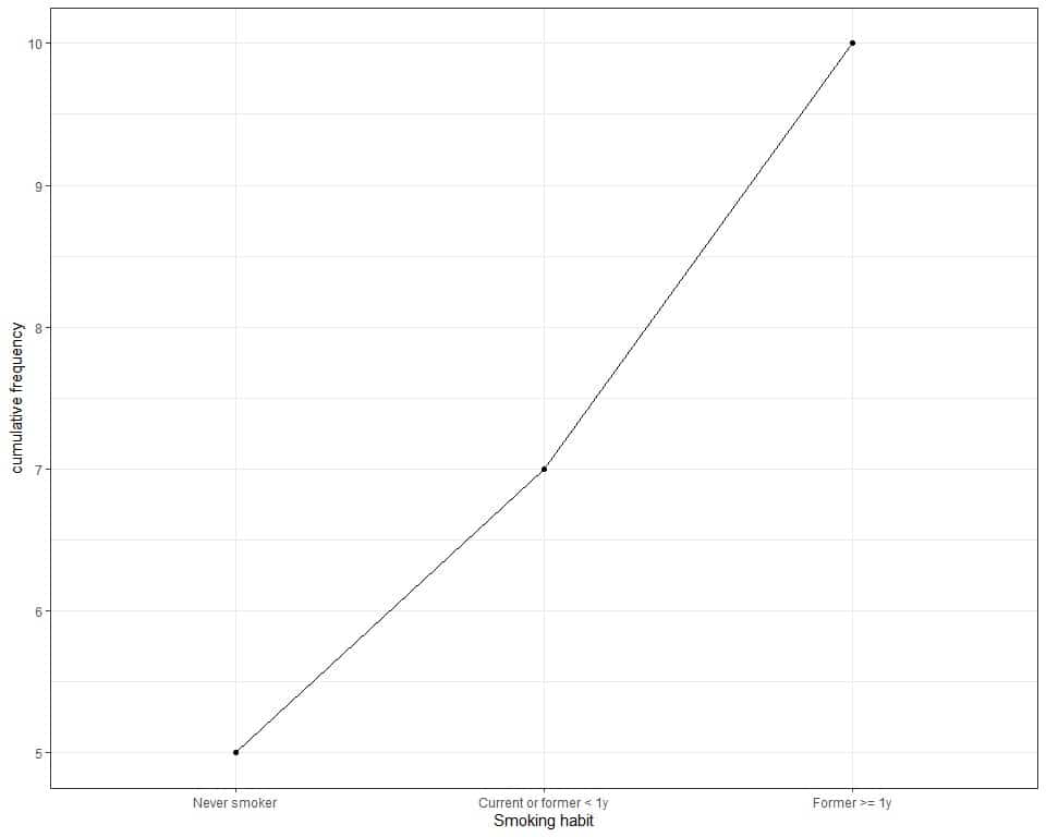
We see that:
- The largest cumulative frequency is 10 so our data points are 10 or 10 participants.
- The cumulative frequency of the first category, never smoker, is 5. This means that its frequency is 5.
- The cumulative frequency of the second category, Current or former < 1y, is 7. This means that the total frequency of never smokers and Current or former < 1y smokers is 7. The individual frequency of the current or former < 1y smokers = current cumulative frequency – previous cumulative frequency = 7-5 = 2.
- The cumulative frequency of the last category, Former >= 1y, is 10. This means that the total frequency of never smokers, Current or former < 1y smokers, and Former >= 1y is 10. The individual frequency of the Former >= 1y smokers is 10-7 = 3.
– Example 2 of categorical data
The following is the frequency table for the marital status of 100 participants from a certain survey.
marital status | frequency |
No answer | 0 |
Never married | 29 |
Separated | 1 |
Divorced | 14 |
Widowed | 20 |
Married | 36 |
We see that the most frequent marital status is “Married” with 36 occurrences.
We can add a third column for the cumulative frequency.
marital status | frequency | cumulative frequency |
No answer | 0 | 0 |
Never married | 29 | 29 |
Separated | 1 | 30 |
Divorced | 14 | 44 |
Widowed | 20 | 64 |
Married | 36 | 100 |
- The cumulative frequency for the first marital status “No answer” is the same as its frequency = 0.
- The cumulative frequency for the second marital status “Never married” = frequency of first marital status + frequency of second marital status = 0+29 = 29.
- The cumulative frequency for the third marital status “Separated” = frequency of first marital status + frequency of second marital status + frequency of third marital status = 0+29+1 = 30.
- The cumulative frequency for the fourth marital status “Divorced” = frequency of first marital status + frequency of second marital status + frequency of third marital status+ frequency of fourth marital status = 0+29+1+14 = 44, and so on.
- The last number of cumulative frequency is the same as the total data points which are 100.
The following line graph can be used to plot the cumulative frequency.
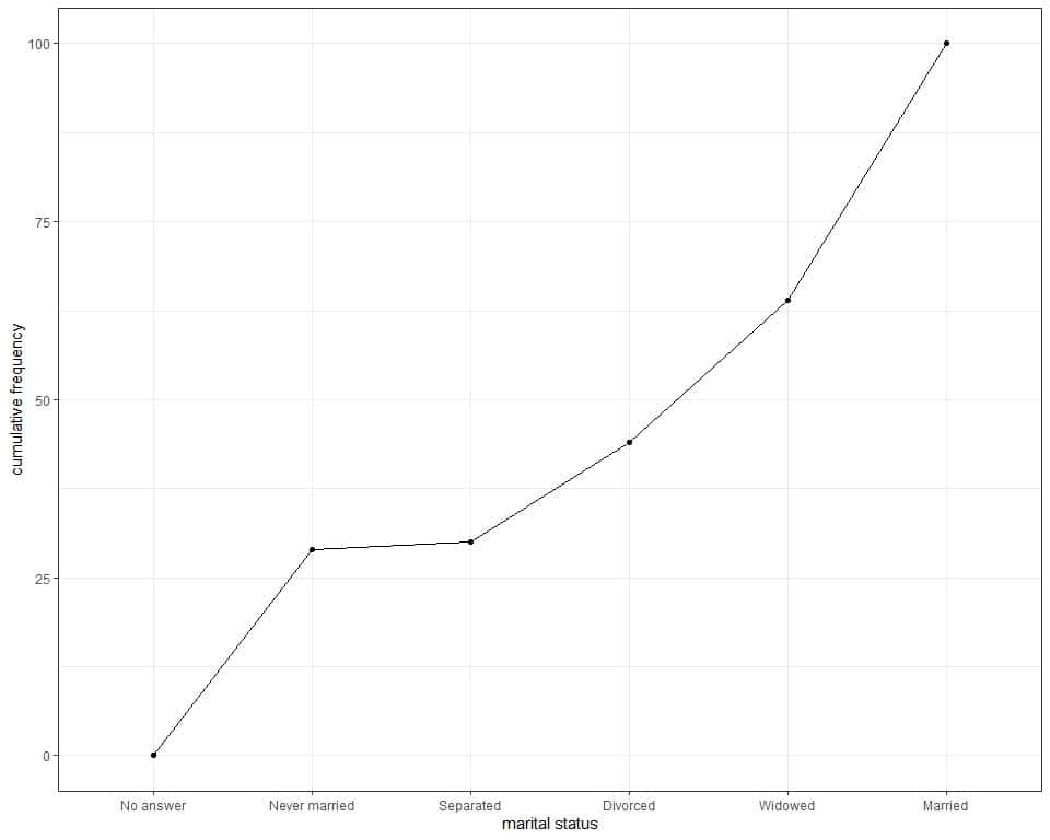
We see the same information that we concluded from the table.
– Example 3 of numerical data
The following is the frequency table for the number of cylinders of 32 different car models in 1973-1974.
Number of cylinders | frequency |
4 | 11 |
6 | 7 |
8 | 14 |
We see that the most frequent number of cylinders is 8 with 14 occurrences or 14 different cars have this number of cylinders. The least frequent number is 6 with only 6 cars having this number.
We can add a third column for the cumulative frequency.
Number of cylinders | frequency | cumulative frequency |
4 | 11 | 11 |
6 | 7 | 18 |
8 | 14 | 32 |
- The cumulative frequency for the first number of cylinders “4” is the same as its frequency = 11.
- The cumulative frequency for the second number “6” = frequency of 4 + frequency of 6 = 11+7 = 18.
- The cumulative frequency for the third number “8” = frequency of 4 + frequency of 6 + frequency of 8 = 11+7+14 = 32.
- The last number of cumulative frequency is the same as the total data points which are 100.
The following line graph can be used to plot the cumulative frequency.
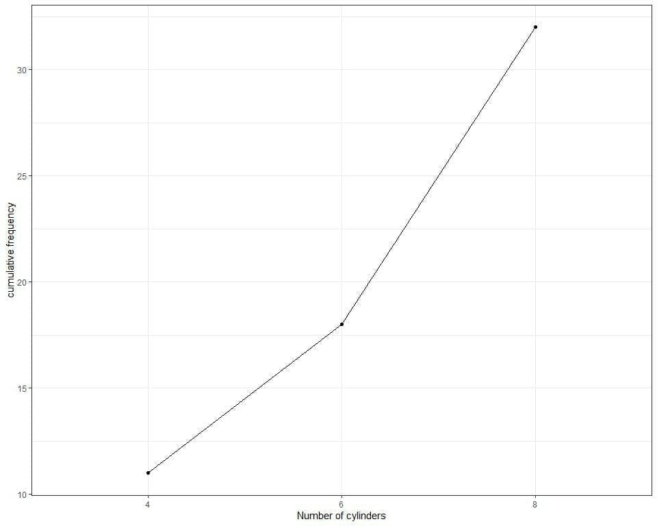
We see the same information that we concluded from the table.
– Example 4 of numerical data
The following is the frequency table for the weights of 100 participants (in Kg) from a certain survey.
Weight | frequency |
43.5 | 1 |
45.8 | 1 |
49 | 1 |
50.4 | 1 |
51 | 1 |
53 | 3 |
53.6 | 1 |
54 | 1 |
55 | 2 |
55.5 | 1 |
55.8 | 1 |
56.4 | 1 |
56.6 | 1 |
56.8 | 1 |
57 | 1 |
58 | 1 |
59 | 1 |
60 | 2 |
60.3 | 1 |
61 | 2 |
62 | 1 |
63 | 1 |
63.4 | 1 |
64 | 3 |
65 | 2 |
65.5 | 1 |
66 | 4 |
67 | 4 |
67.5 | 1 |
68 | 3 |
69 | 4 |
70 | 5 |
71 | 1 |
71.5 | 1 |
72 | 2 |
72.4 | 1 |
73 | 2 |
74 | 1 |
75 | 4 |
75.4 | 1 |
76 | 4 |
77 | 3 |
78 | 1 |
79 | 4 |
79.2 | 1 |
80 | 2 |
80.2 | 1 |
80.4 | 1 |
84 | 1 |
84.5 | 1 |
84.6 | 1 |
85 | 1 |
87.5 |
|
|
|
89 | 2 |
91.8 | 1 |
94 | 3 |
95.5 | 1 |
98 | 1 |
We can add a third column for the cumulative frequency.
Weight | frequency | cumulative frequency |
43.5 | 1 | 1 |
45.8 | 1 | 2 |
49 | 1 | 3 |
50.4 | 1 | 4 |
51 | 1 | 5 |
53 | 3 | 8 |
53.6 | 1 | 9 |
54 | 1 | 10 |
55 | 2 | 12 |
55.5 | 1 | 13 |
55.8 | 1 | 14 |
56.4 | 1 | 15 |
56.6 | 1 | 16 |
56.8 | 1 | 17 |
57 | 1 | 18 |
58 | 1 | 19 |
59 | 1 | 20 |
60 | 2 | 22 |
60.3 | 1 | 23 |
61 | 2 | 25 |
62 | 1 | 26 |
63 | 1 | 27 |
63.4 | 1 | 28 |
64 | 3 | 31 |
65 | 2 | 33 |
65.5 | 1 | 34 |
66 | 4 | 38 |
67 | 4 | 42 |
67.5 | 1 | 43 |
68 | 3 | 46 |
69 | 4 | 50 |
70 | 5 | 55 |
71 | 1 | 56 |
71.5 | 1 | 57 |
72 | 2 | 59 |
72.4 | 1 | 60 |
73 | 2 | 62 |
74 | 1 | 63 |
75 | 4 | 67 |
75.4 | 1 | 68 |
76 | 4 | 72 |
77 | 3 | 75 |
78 | 1 | 76 |
79 | 4 | 80 |
79.2 | 1 | 81 |
80 | 2 | 83 |
80.2 | 1 | 84 |
80.4 | 1 | 85 |
84 | 1 | 86 |
84.5 | 1 | 87 |
84.6 | 1 | 88 |
85 | 1 | 89 |
87.5 | 1 | 90 |
88 | 2 | 92 |
89 | 2 | 94 |
91.8 | 1 | 95 |
94 | 3 | 98 |
95.5 | 1 | 99 |
98 | 1 | 100 |
- The cumulative frequency increases to reach 100.
The following line graph can be used to plot the cumulative frequency.
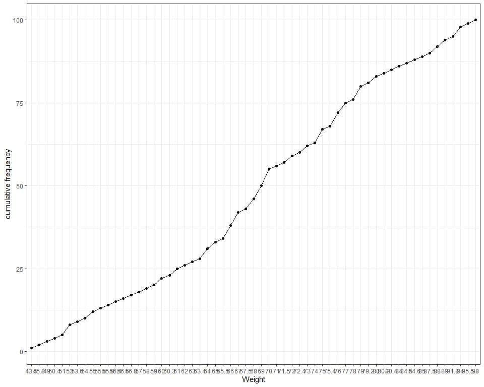
We see that the frequency table is too long and non-informative as we have many different weight values. Also, the plot has many crowded x-axis values.
In that case, we use a bin frequency table. The bin frequency table groups values into equal-sized bins and each bin includes a range of values.
range | frequency |
43.5 – 53.5 | 8 |
53.5 – 63.5 | 20 |
63.5 – 73.5 | 34 |
73.5 – 83.5 | 23 |
83.5 – 93.5 | 10 |
93.5 – 103.5 | 5 |
Here we group the data or weights into 6 equal-sized bins. Each bin includes a range of 10 values.
For example, the bin “43.5-53.5” includes weights from 43.5 to 53.5 Kg.
The bin “53.5-63.5” includes values larger than 53.5 Kg to 63.5 Kg and so on.
We can add a third column for the cumulative frequency.
range | frequency | cumulative frequency |
43.5 – 53.5 | 8 | 8 |
53.5 – 63.5 | 20 | 28 |
63.5 – 73.5 | 34 | 62 |
73.5 – 83.5 | 23 | 85 |
83.5 – 93.5 | 10 | 95 |
93.5 – 103.5 | 5 | 100 |
The cumulative frequency increases to reach 100.
If we plot the cumulative frequency as a line graph.
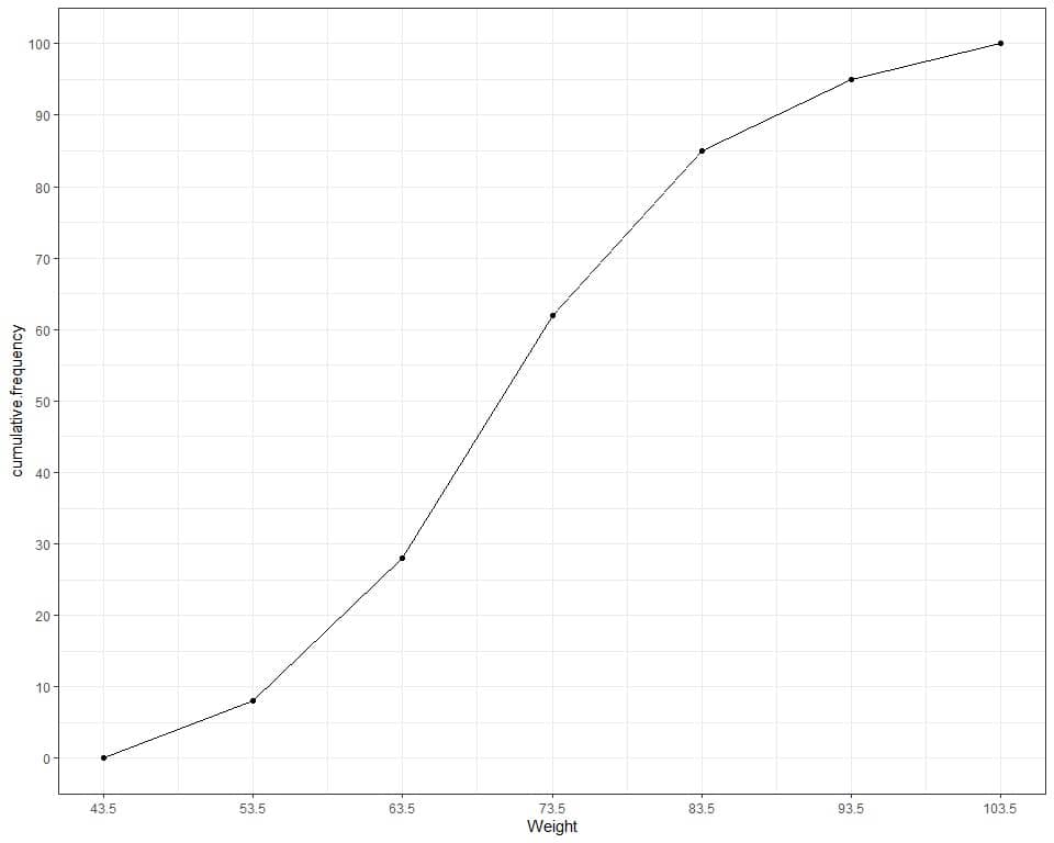
We see from the table or graph that:
- None of the 100 participants has a weight less than 43.5 kg since the cumulative frequency at 43.5 kg is 0.
- Less than 10 participants (or 8) have weight less than or equal to 53.5 kg.
- Less than 30 participants (or 28) have weight less than or equal to 63.5 kg.
- 85 participants are having a weight less than or equal to 83.5 kg.
How to find cumulative frequency?
– Example 1 of categorical data
The following is the frequency table for the reported income category of 100 participants from a certain survey.
Income | frequency |
Lt $1000 | 1 |
$1000 to 2999 | 3 |
$3000 to 3999 | 4 |
$4000 to 4999 | 0 |
$5000 to 5999 | 1 |
$6000 to 6999 | 0 |
$7000 to 7999 | 1 |
$8000 to 9999 | 5 |
$10000 – 14999 | 13 |
$15000 – 19999 | 6 |
$20000 – 24999 | 13 |
$25000 or more | 53 |
- “Lt $1000” means less than 1000.
To calculate the cumulative frequency for each category:
1. Add a third column named “cumulative frequency”.
Income | frequency | cumulative frequency |
Lt $1000 | 1 | |
$1000 to 2999 | 3 |
|
$3000 to 3999 | 4 |
|
$4000 to 4999 | 0 |
|
$5000 to 5999 | 1 |
|
$6000 to 6999 | 0 |
|
$7000 to 7999 | 1 |
|
$8000 to 9999 | 5 |
|
$10000 – 14999 | 13 |
|
$15000 – 19999 | 6 |
|
$20000 – 24999 | 13 |
|
$25000 or more | 53 |
|
2. The cumulative frequency for the first category “Lt $1000” is the same as the frequency so it is 1.
- The cumulative frequency for the second category “$1000 to 2999” = frequency of first category + frequency of second category = 1+3 = 4.
- The cumulative frequency for the third category “$3000 to 3999” = frequency of first category + frequency of second category + frequency of third category = 1+3+4 = 8.
- The cumulative frequency for the fourth category “$4000 to 4999” = frequency of first category + frequency of second category + frequency of third category + frequency of fourth category = 1+3+4+0 = 8.
Income | frequency | cumulative frequency |
Lt $1000 | 1 | 1 |
$1000 to 2999 | 3 | 4 |
$3000 to 3999 | 4 | 8 |
$4000 to 4999 | 0 | 8 |
$5000 to 5999 | 1 |
|
$6000 to 6999 | 0 |
|
$7000 to 7999 | 1 |
|
$8000 to 9999 | 5 |
|
$10000 – 14999 | 13 | |
$15000 – 19999 | 6 |
|
$20000 – 24999 | 13 |
|
$25000 or more | 53 |
|
3. Continue till completing all the rows. The last number must be 100 which the sample size or number of participants.
Income | frequency | cumulative frequency |
Lt $1000 | 1 | 1 |
$1000 to 2999 | 3 | 4 |
$3000 to 3999 | 4 | 8 |
$4000 to 4999 | 0 | 8 |
$5000 to 5999 | 1 | 9 |
$6000 to 6999 | 0 | 9 |
$7000 to 7999 | 1 | 10 |
$8000 to 9999 | 5 | 15 |
$10000 – 14999 | 13 | 28 |
$15000 – 19999 | 6 | 34 |
$20000 – 24999 | 13 | 47 |
$25000 or more | 53 | 100 |
4. To plot this cumulative frequency as a line graph, plot the categories on the x-axis and cumulative frequency on the y-axis.
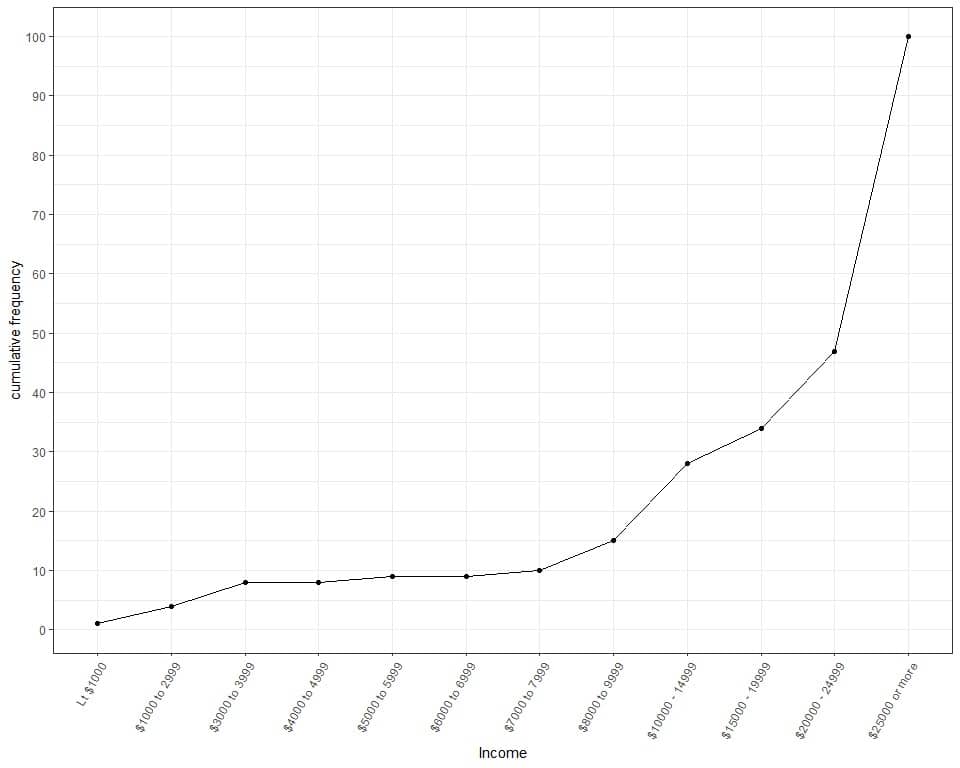
We see from the table or graph that :
- The upper boundary of cumulative frequency is 100 because our sample size is 100.
- Less than 10 participants (or 8) earn an income up to 3999.
- Less than 30 participants (or 28) earn an income up to 14,999.
- Less than 50 participants (or 47) earn an income up to 24,999 and more than 50 participants (or 100-47 = 53) earn the highest income category (25,000 or more).
– Example 2 of numerical data with repeated values
The following is the frequency table for the number of forward gears of 32 different car models in 1973-1974.
gear | frequency |
3 | 15 |
4 | 12 |
5 | 5 |
To calculate the cumulative frequency for each number:
1. Add a third column named “cumulative frequency”.
gear | frequency | cumulative frequency |
3 | 15 | |
4 | 12 |
|
5 | 5 |
|
2. The cumulative frequency for the first number “3” is the same as its frequency so it is 15.
- The cumulative frequency for the second number “4” = frequency of first number + frequency of second number = 15+12 = 27.
- The cumulative frequency for the third number “5” = frequency of first number + frequency of second number + frequency of third number = 15+12+5 = 32.
- The last number must be 32 which the sample size or number of cars.
gear | frequency | cumulative frequency |
3 | 15 | 15 |
4 | 12 | 27 |
5 | 5 | 32 |
3. To plot this cumulative frequency as a line graph, plot the numbers on the x-axis and cumulative frequency on the y-axis.
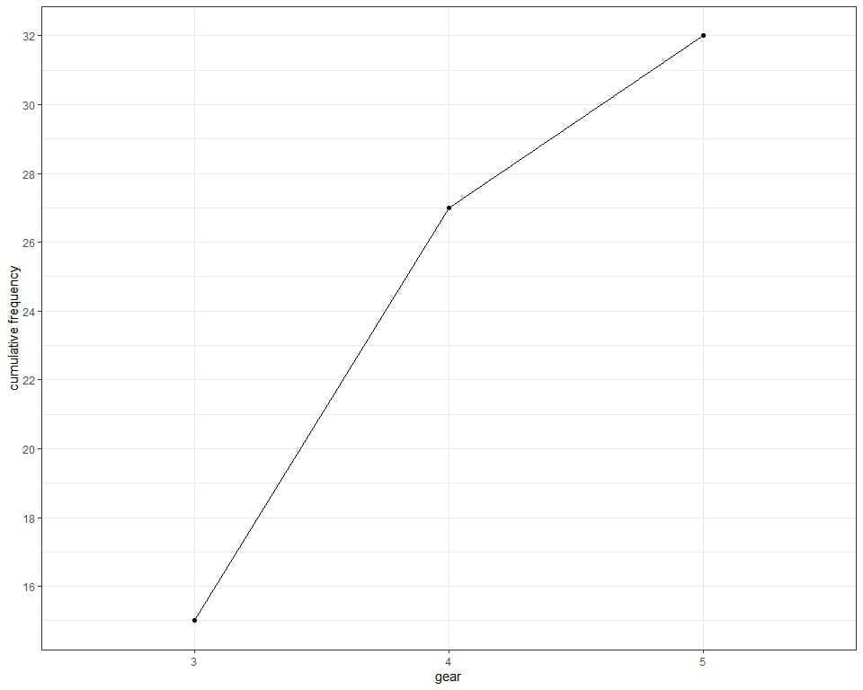
We see from the table or graph that:
- The upper boundary of cumulative frequency is 32 because our sample size is 32.
- No cars have gears less than 3.
- 15 cars have 3 gears.
- 27 cars have gears up to 4. To obtain the individual frequency of the number 4 = current cumulative frequency – previous cumulative frequency = 27-15 = 12.
- 32 cars have gears up to 5. To obtain the individual frequency of the number 5 = current cumulative frequency – previous cumulative frequency = 32-27 = 5.
– Example 3 of numerical data with the bin frequency table
The following is the bin frequency table for the age (in years) of 200 participants from a certain survey.
range | frequency |
19 – 31 | 35 |
31 – 43 | 48 |
43 – 55 | 60 |
55 – 67 | 24 |
67 – 79 | 18 |
79 – 91 | 15 |
- If you sum these numbers, you will get 200 which is the total number of data. 35+48+60+24+18+15 = 200.
- The bin “19-31” includes ages from 19 to 31 years.
- The bin “31-43” includes ages larger than 31 years to 43 years.
- The bin “43-55” includes ages larger than 43 years till 55 years, and so on.
To calculate the cumulative frequency for each frequency:
1. Add a third column named “cumulative frequency”.
range | frequency | cumulative frequency |
19 – 31 | 35 |
|
31 – 43 | 48 | |
43 – 55 | 60 |
|
55 – 67 | 24 | |
67 – 79 | 18 |
|
79 – 91 | 15 |
|
2. Add an imaginary first bin with 0 frequency.
- Determine the class width = 31-19 = 12.
- Subtract this class width from the lower limit of the first range to obtain the range for the imaginary first bin. 19-12 = 7.
- The range for the imaginary first bin is “7-19”.
range frequency cumulative frequency
range | frequency | cumulative frequency |
7-19 | 0 |
|
19 – 31 | 35 | |
31 – 43 | 48 |
|
43 – 55 | 60 | |
55 – 67 | 24 |
|
67 – 79 | 18 | |
79 – 91 | 15 |
|
3. Calculate the cumulative frequency as we do before.
- The cumulative frequency for the first range “7-19” is the same as its frequency or 0.
- The cumulative frequency for the second range “19-31” = frequency of first range + frequency of second range = 0+35 = 35.
- The cumulative frequency for the third range “31-43” = frequency of first range + frequency of second range + frequency of third range = 0+35+48 = 83, and so on.
- The last cumulative frequency must be 200 which is the sample size or the number of participants.
range | frequency | cumulative frequency |
7-19 | 0 | 0 |
19 – 31 | 35 | 35 |
31 – 43 | 48 | 83 |
43 – 55 | 60 | 143 |
55 – 67 | 24 | 167 |
67 – 79 | 18 | 185 |
79 – 91 | 15 | 200 |
4. To plot the cumulative frequency as a line graph, plot the upper border of each range on the x-axis and the cumulative frequency on the y-axis.
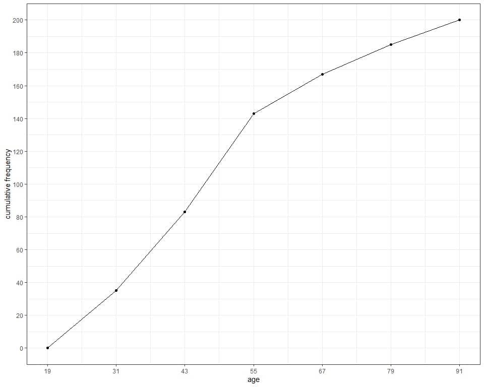
We see from the table or graph that :
- None of the 200 participants aged less than 19 years since the cumulative frequency at 19 years is 0.
- Less than 40 participants (or 35) have age less than or equal to 31 years.
- Less than 150 participants (or 143) have age less than or equal to 55 years.
- 185 participants have age less than or equal to 79 years. So, the remaining 15 participants have an age of more than 79 years in our sample.
Cumulative frequency formula
From the above examples, we see that the formula for cumulative frequency is:
Cumulative frequency = Current frequency + sum of previous frequencies = current frequency + previous cumulative frequency.
Practical questions
1. The following cumulative frequency table lists the cumulative frequency of different religions for 150 persons.
Religion | cumulative frequency |
No answer | 0 |
Don’t know | 0 |
Inter-nondenominational | 2 |
Native american | 3 |
Christian | 9 |
Orthodox-christian | 10 |
Moslem/islam | 10 |
Other eastern | 10 |
Hinduism | 11 |
Buddhism | 11 |
Other | 14 |
None | 40 |
Jewishц | |
Protestant | 150 |
Not applicable | 150 |
Why is the cumulative frequency for the first two categories, “No answer” and “Don’t know” zero?
What is the frequency for Christian in this data?
What is the frequency for Buddhism in this data?
2. The following is the cumulative frequency table for the hours per day watching TV for the 100 persons.
TV | cumulative frequency |
0 | 6 |
1 | 27 |
2 | 51 |
3 | 70 |
4 | 83 |
5 | 89 |
7 | 92 |
8 | 95 |
10 | 96 |
12 | 100 |
How many persons are not watching TV in this data?
How many persons are watching TV for up to 5 hours per day?
3. The following cumulative frequency plot draws the cumulative frequency of different classifications for 100 different storms.
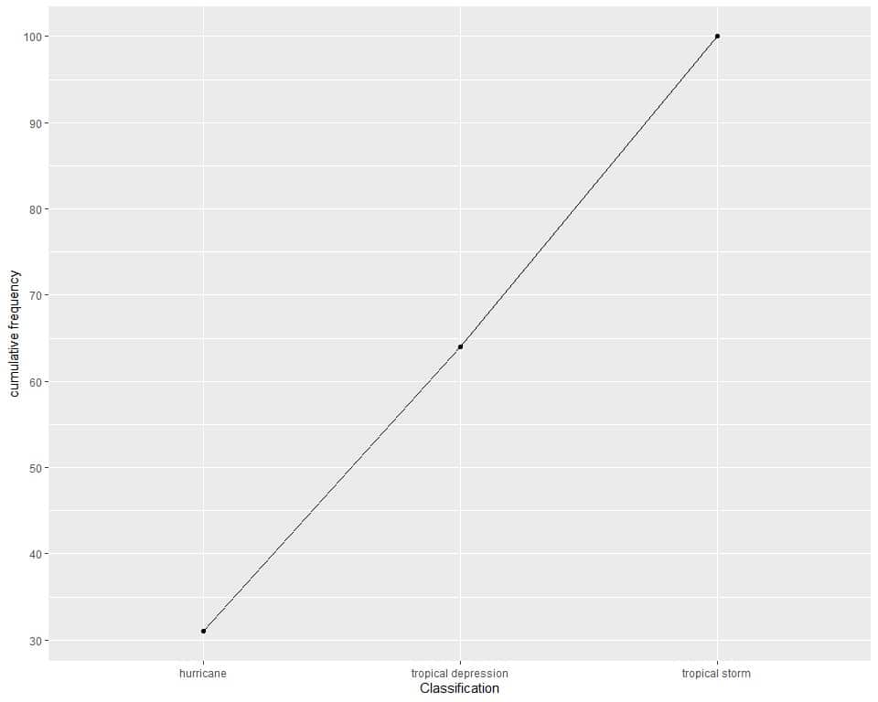
How many storms are either hurricane or tropical depression (approximately)?
4. The following is a cumulative frequency table for the prices of 200 different diamonds.
range | cumulative frequency |
300 – 800 | 90 |
800 – 1300 | 90 |
1300 – 1800 | 90 |
1800 – 2300 | 90 |
2300 – 2800 | 200 |
How many diamonds have prices up to 1,300?
How many diamonds have prices up to 2,300?
If the answer to both questions is the same, why?
5. The following is a cumulative frequency plot for the daily temperature measurements in New York, May to September 1973.
How many days are recorded in this data (approximately)?
How many days in this data have temperatures up to 85 (approximately)?
Answers
1. The cumulative frequency for both “No answer” and “Don’t know” is zero because they have zero frequency in the data.
The frequency for Christian in this data = current cumulative frequency – previous cumulative frequency = 9-3 = 6.
Similarly, the frequency for Buddhism in this data = 11-11 = 0.
2. The first row is for 0 tv hours or not watching TV with 6 cumulative frequency, so 6 persons in that data do not watch TV.
Look at row 5, we see 89 persons who watch TV for up to 5 hours per day.
3. The point for the cumulative frequency of hurricane and tropical depression storms is slightly below the 65 line, so it is nearly 64.
4. The number of diamonds that have priced up to 1,300 is 90.
The number of diamonds that have priced up to 2,300 is 90 also.
The previous bin “300-800” has 90 cumulative frequency. This means that both of these bins “800-1300” and “1800-2300” have zero frequency.
5. The upper point of cumulative frequency is nearly 150 or 150 days.
The cumulative frequency at 85 is nearly 120 or 120 days.