Derivative test – Types, Explanation, and Examples
Derivative tests are applications of derivatives that help us determine whether a critical number is a local maximum or minimum. Learning about the
first and second derivative tests will help us confirm a critical number’s nature without graphing the actual function.
The first and second derivative tests allow us to determine a function’s potential critical numbers and local extrema. These two tests tell us whether the function is concaving upward or downward within a given interval.By the end of this article, you should be able to:
- Finding the critical numbers of a function using its first derivative.
- Use the two derivative tests to confirm if a critical number is a local extremum.
- Know the difference between the two derivative tests.
These two derivative tests will also lay out the foundation for other applications and properties we’ll learn in our calculus classes. Hence, this is going to be a discussion filled with concepts and rules. Take notes when possible and apply what you’ve learned in the problems we’ve prepared just for you.
What is the first derivative test?
The first derivative test allows us to find the intervals where the
function is increasing or decreasing. This derivative also helps us
find the local maxima and minima of a function.According to the first derivative test, when $c$ is a critical number of $f(x)$, we can observe the following:
- When $f’(x)$ switches from negative to positive at $c$, $f(x)$ has a local (or relative) minimum at $(c, f(c))$.
- Similarly, when $f’(x)$ switches from positive to negative at $c$, $f(x)$ has a local (or relative) maximum at $(c, f(c))$.
- If the sign of $f’(x)$ remains the same on both sides of $c$, $f(x)$ has no extremum at $(c, f(c))$.
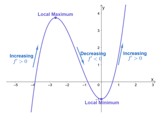
The graph of $y = 0.5 x^(3)+2 x^(2)-1$ is as shown above. This function has critical numbers at $x = -\dfrac{8}{3}$ and $x = 0$. Let’s take a look at the signs of $f’(x)$ as we approach each critical number from the left and right.
- At $x = -\dfrac{8}{3}$, we can see that $f’(x)$’s sign changes from positive to negative, so we have a local maximum at $x = -\dfrac{8}{3}$.
- Similarly, $f’(x)$’s sign changes from negative to positive at $x =0$, so we have a local minimum at $x = 0$.
These conditions hold true as long as $f(x)$ is a continuous function. We can also confirm local extremums without the graph and we’ll learn more about that in the next section.
How to do the first derivative test?
We will still use the conditions discussed in our earlier discussion of the first derivative test. These steps will guide you in applying this method correctly:
- Find the critical numbers of $x$ by equating $f’(x)$ to $0$.
- Divide the domain of $f(x)$ into smaller intervals containing the critical numbers as bounds.
- Use a test point for each interval and observe the sign of $f’(x)$.
- Use these results and the first derivative test’s conditions to determine whether the function has a local maximum or minimum.
Let’s apply these steps to find the local extrema of $f(x) = 5x^2 -8x + 1$. Begin by finding the values of $x$ where $f’(x) = 0$. Use the
derivative rules to find the expression for f’(x)$.\begin{aligned}f(x)&= 2x^2 -8x + 1\\f'(x) &=\dfrac{d}{dx}2x^2 -\dfrac{d}{dx}8x + \dfrac{d}{dx}1,\phantom{x}\color{Teal}\text{Difference & Sum Rules}\\&= {\color{Teal}2\dfrac{d}{dx}x^2 – 8\dfrac{d}{dx}x} +{\color{Orchid}0},\phantom{x}{\color{Teal}\text{Constant Multiple Rule}}\text{ & } {\color{Orchid}\text{Cosntant Rule}}\\&= 2{\color{Teal}(2x)}-8{\color{Teal}(1)},\phantom{x}{\color{Teal}\text{Power Rule}}\\&=4x -8\end{aligned}Equate $f’(x)$ to zero to find the critical number of $f(x)$.\begin{aligned}4x – 8 &=0 \\4x &= 8\\x&= 2\end{aligned}The domain of $f(x)$ is $(-\infty, \infty)$, so divide this into smaller intervals to check the behavior of $f(x)$ in between $x = 2$. Assign a test value to check the sign of $f’(x)$ for each interval.
| Interval | Test Value | Sign of $\boldsymbol{f’(x)}$ | Conclusion |
| \begin{aligned}\boldsymbol{(-\infty, 2)}\end{aligned} | \begin{aligned}x&=1\end{aligned} | \begin{aligned}-\end{aligned} | $f(x)$ is decreasing |
| \begin{aligned}\boldsymbol{(2, \infty)}\end{aligned} | \begin{aligned}x&=3\end{aligned} | \begin{aligned}+\end{aligned} | $f(x)$ is increasing |
From the table, we can see that $f’(x)$’s sign changed from negative to positive. This means that $x = 2$ is located at the minimum point of $f(x)$.\begin{aligned}c &= 2\\f(c) &= 2(2)^2 – 8(2) + 1\\&= -7\end{aligned}This means that $f(x)$ has a minimum point at $(2, -7)$.The graph $f(x) = 2x^2 – 8x + 1$ is shown below to confirm this.

This also confirms how vertices represent a quadratic function’s extremum. Apply the same steps we’ve used to find other function’s extremum. Don’t worry, you’ll be able to use the first derivative test in our example section later! For now, let’s move on to our next derivative test: the second derivative test.
What is the second derivative test?
The second derivative test comes in handy when we have twice differentiable functions (meaning, we can take the derivative $f(x)$ twice in a row). We can confirm the relative maxima using $f”(x)$.
- When $\boldsymbol{f”(x) >0}$, the function has a local minimum at $(c, f(c))$.
- When $\boldsymbol{f”(x) <0}$, the function has a local maximum at $(c, f(c))$.
- When $\boldsymbol{f”(x) =0}$, the second derivative test will not be helpful. Use the first derivative test instead.

Here’s an example of a function ($f(x) = x^5 -2x^3$) with two local extremums. We can confirm this by observing the signs of $f”(x)$ at these two critical points.
- At $x =-1.02$, the double derivative of $f(x)$ is negative, so $(-1.02, 1.08)$ is the function’s relative maximum.
- Similarly, since $f”(x) > 0$ at $x =1.10$, the point $(1.10, -1.05)$ is a relative minimum.
This also shows us that when $f”(x)$
is less than zero, the function is
concaving downwards. Similarly, when $f”(x)$
is greater than zero, the function is
concaving upward.
How to do the second derivative test?
The good thing about the second derivative test is that we’ll only evaluate $f”(x)$ at $c$ as opposed to the first derivative test. Keep these steps in mind when applying the second derivative test to check for relative extremums:
- Differentiate $f(x)$ and equate $f’(x)$ to zero to find the function’s critical numbers.
- Differentiate $f’(x)$ this time to find the second derivative of $f(x)$.
- Substitute $x = c$ or the critical numbers of $f(x)$ into the expression of $f”(x)$.
- Observe the signs and use the conditions we’ve learned to confirm whether $x=c$ is a local maximum or minimum.
Why don’t we go ahead and confirm the local extremums of $f(x) = x^5 -2x^3$ using these steps? First, take the derivative of $f(x)$ using the fundamental derivative rules we’ve learned in the past.\begin{aligned}f(x)&= x^5 -2x^3\\f'(x) &=\dfrac{d}{dx}x^5 – \dfrac{d}{dx}2x^3,\phantom{x}\color{Teal}\text{Difference Rule}\\&= \dfrac{d}{dx}x^5 -{\color{Teal}2\dfrac{d}{dx}x^3 },\phantom{x}{\color{Teal}\text{Constant Multiple Rule}}\\&={\color{Teal}(5x^4)}-2{\color{Teal}(3x^2)},\phantom{x}{\color{Teal}\text{Power Rule}}\\&= 5x^4-6x^2\end{aligned}Find the critical numbers by equation $f’(x)$ to zero.
All values that satisfy this equation will be considered a critical number.\begin{aligned}f'(x) &=0\\5x^4-6x^2&=0\\x^2(5x^2 -6) &=0\\x&=0\\5x^2 – 6&=0\\5x^2&= 6\\x^2&= \dfrac{6}{5}\\x&= \pm \sqrt{\dfrac{6}{5}}\end{aligned}Now, differentiate $f’(x)$ once more and then substitute these three values into the resulting expression.\begin{aligned}f'(x) &=5x^4-6x^2\\f”(x)&=\dfrac{d}{dx}5x^4 – \dfrac{d}{dx}6x^2,\phantom{x}\color{Teal}\text{Difference Rule}\\&= {\color{Teal}5\dfrac{d}{dx}x^4} -{\color{Teal}6\dfrac{d}{dx}x^2},\phantom{x}{\color{Teal}\text{Constant Multiple Rule}}\\&=5{\color{Teal}(4x^3)}-6{\color{Teal}(2x)},\phantom{x}{\color{Teal}\text{Power Rule}}\\&= 20x^3-12x\end{aligned}The table below summarizes the result when we substitute $x =\left\{-\sqrt{\dfrac{6}{5}},0,\sqrt{\dfrac{6}{5}}\right\}$ into $f”(x)$.
| Critical Numbers | Sign of $\boldsymbol{f’’(x)}$ | Conclusion |
| \begin{aligned}x = -\sqrt{\dfrac{6}{5}}\end{aligned} | \begin{aligned}-\end{aligned} | Local Maximum |
| \begin{aligned}x = 0\end{aligned} | \begin{aligned}0\end{aligned} | No conclusion |
| \begin{aligned}x =\sqrt{\dfrac{6}{5}}\end{aligned} | \begin{aligned}+\end{aligned} | Local Minimum |
From the signs of $f”\left(-\sqrt{\dfrac{6}{5}}\right)$ and $f”\left(\sqrt{\dfrac{6}{5}}\right)$, we can conclude that they are local extremums of $f(x)$. In fact, $f”\left(-\sqrt{\dfrac{6}{5}}\right)$ is a local maximum while $f”\left(\sqrt{\dfrac{6}{5}}\right)$ is a local minimum.
Summarizing the two derivative tests
We’ve discussed the first and second derivative tests, so we’ll summarize and do a quick recap of what we’ve learned so far.
- In the first derivative test, $(c, f(c))$ is a local extremum when $f’(x)$ changes sign.
- When $f’(x)$’s sign changes from negative to positive, $(c, f(c))$ is a local minimum.
- When $f’(x)$’s sign changes from positive to negative, $(c, f(c))$ is a local maximum.
- As for the second derivative test, $(c, f(c))$ will depend on $f”(c)$’s sign.
- When $f”(c)<0$, the point $(c, f(c))$ is a local maximum.
- When $f”(c)>0$, the point $(c, f(c))$ is a local minimum.
The table below will help also help us predict the function’s behavior and curve depending on its first and second derivative’s signs.
| Observing the First and Second Derivative’s Signs | Function’s Behavior | Shape of Function’s Curve |
| \begin{aligned}f’(x)&>0\\ f”(x) &> 0\end{aligned} | $f(x)$ is increasing | $f(x)$ is concaving upward |
| \begin{aligned}f’(x)&<0\\ f”(x) &> 0\end{aligned} | $f(x)$ is decreasing | $f(x)$ is concaving upward |
| \begin{aligned}f’(x)&>0\\ f”(x) &< 0\end{aligned} | $f(x)$ is increasing | $f(x)$ is concaving downward |
| \begin{aligned}f’(x)&<0\\ f”(x) &> 0\end{aligned} | $f(x)$ is decreasing | $f(x)$ is concaving downward |
These are the concepts that you’ll need to answer the problems shown below. Keep these pointers in mind when answering our sample problems!
Example 1Let’s say we have the function, $f(x) = \dfrac{x^2 – 6x +9}{x^2 -4}$, find the following:a. The critical numbers of $f(x)$.
b. The local extrema of $f(x)$ using the first derivative test.
c. The intervals where $f(x)$ is increasing and decreasing.
SolutionWe begin by differentiating $\dfrac{x^2 – 6x +9}{x^2 -4}$ using the
quotient rule and other derivative rules as shown below.\begin{aligned}f(x) &=\dfrac{x^2 -6x +9}{x^2 -4}\\f'(x)&=\dfrac{(x^2 -4)\dfrac{d}{dx}(x^2-6x+9)-(x^2-6x+9)\dfrac{d}{dx}(x^2 -4)}{(x^2 -4)^2},\phantom{x}\color{Teal}\text{Quotient Rule}\\&=\dfrac{(x^2 -4){\color{Teal}\left(\dfrac{d}{dx}x^2-\dfrac{d}{dx}6x+\dfrac{d}{dx}9\right)}-(x^2-6x+9){\color{Teal}\left(\dfrac{d}{dx}x^2 -\dfrac{d}{dx}4\right)}}{(x^2 -4)^2},\phantom{x}\color{Teal}\text{Sum & Difference Rules}\\&=\dfrac{(x^2 -4)\left(\dfrac{d}{dx}x^2-{\color{Teal}6\dfrac{d}{dx}x}+{\color{Orchid}0}\right)-(x^2-6x+9)\left(\dfrac{d}{dx}x^2 -{\color{Orchid}0}\right)}{(x^2 -4)^2},\phantom{x}{\color{Teal} \text{Constant Multiple Rule}}\text{ & }{\color{Orchid}\text{Constant Rule}}\\&= \dfrac{(x^2 -4)[{\color{Teal}2x} – 6({\color{Teal}1})]-(x^2-6x+9)({\color{Teal}2x} )}{(x^2 -4)^2},\phantom{x}\color{Teal}\text{Power Rule}\end{aligned}Simplify the expression for $f’(x)$ by algebraic manipulation then equate the resulting expression to $0$. This will lead us to the value of $x$ where $f(x)$ is an extremum.\begin{aligned}f'(x)&= \dfrac{(x^2-4)(2x -6)-(x^2-6x+9)(2x)}{(x^2 -4)^2}\\&= \dfrac{2(x^2 -4)(x-3) – (x-3)^2(2x)}{(x^2-4)^2}\\&= \dfrac{2(x-3)[(x^2 -4)-x(x-3)]}{(x^2 -4)^2}\\&= \dfrac{2(x-3)(3x-4)}{(x^2-4)^2}\\\\f'(x)&= 0\\\dfrac{2(x-3)(3x -4)}{(x^2 -4)^2} &= 0\\2(x -3)(3x-4)&=0\\x&= 3\\x&= \dfrac{4}{3}\end{aligned}a. Hence, the critical numbers of $f(x)$ are $x = \dfrac{4}{3}$ and $x =3$.As long as $x \neq \pm 2$, $f(x)$ is valid and continuous. Divide the domain of $f(x)$, $(-\infty, -2) \cup(-2, 2)\cup (2, \infty)$, into smaller intervals to account for the critical numbers. Observe the $f’(x)$’s sign changes between these intervals.
| Interval | Test Value | Sign of $\boldsymbol{f’(x)}$ | Conclusion |
| \begin{aligned}\left (-\infty, -2\right)\end{aligned} | \begin{aligned}x&=-3\end{aligned} | \begin{aligned}+\end{aligned} | $f(x)$ is increasing |
| \begin{aligned} \left(-2, -\dfrac{4}{3}\right)\end{aligned} | \begin{aligned}x&=-1.5\end{aligned} | \begin{aligned}+\end{aligned} | $f(x)$ is increasing |
| \begin{aligned} \left(-\dfrac{4}{3}, 2\right)\end{aligned} | \begin{aligned}x&=1\end{aligned} | \begin{aligned}-\end{aligned} | $f(x)$ is decreasing |
| \begin{aligned} (2, 3)\end{aligned} | \begin{aligned}x&=2.5\end{aligned} | \begin{aligned}-\end{aligned} | $f(x)$ is decreasing |
| \begin{aligned} (3, \infty)\end{aligned} | \begin{aligned}x&=4\end{aligned} | \begin{aligned}+\end{aligned} | $f(x)$ is increasing |
From the results, we can see that $f’(x)$’s sign has changed from positive to negative at $x = \dfrac{4}{3}$. This means that $\left(\dfrac{4}{3}, \left(\dfrac{4}{3}\right)\right)$ is a local maximum. Similarly, $f’(x)$’s signs changed from negative to positive, so $(3, f(3))$ is a local minimum.b. This means that $f(x)$ has a local minimum at $(3, 0)$ and a local maximum at $\left(\dfrac{4}{3}, -\dfrac{5}{4}\right)$.The right-most column tells us the intervals where $f(x)$ is increasing and decreasing.c. Hence, $f(x)$ is increasing at the intervals $(-\infty, -2)$, $\left(-2, -\dfrac{4}{3}\right)$, and $(3, \infty)$. In addition, $f(x)$ is decreasing at the intervals, $\left(-\dfrac{4}{3}, 2\right)$ and $(3, \infty)$.
Example 2Confirm that the function from Example 1 has a local maximum at $x = \dfrac{4}{3}$ and a local minimum at $x = 3$ using the second derivative test. Use these results to determine the intervals where $f(x)$ is concaving upwards and downwards.
SolutionFrom Example 1, we have $f’(x) = \dfrac{2(x-3)(3x -4)}{(x^2 -4)^2}$. We’ve also shown that $x = \dfrac{4}{3}$ and $x = 3$ are $f(x)$’s critical numbers. We can confirm the local extremums of $f(x)$ by taking the derivative of $f’(x)$.First, let’s simplify the numerator of $f’(x)$ then apply the derivative rules as shown below.\begin{aligned}f'(x)&= \dfrac{2(x-3)(3x -4)}{(x^2 -4)^2} \\&= \dfrac{6x^2 – 26x + 24}{(x^2 -4)^2}\\\\f”(x)&= \dfrac{(x^2 -4)^2 \dfrac{d}{dx}(6x^2 – 26x + 24) – (6x^2 – 26x + 24)\dfrac{d}{dx}(x^2-4)^2}{(x^2 -4)^4},\phantom{x}{\color{Teal}\text{Quotient Rule}}\\&= \dfrac{(x^2 -4)^2 {\color{Teal}\left(\dfrac{d}{dx}6x^2 – \dfrac{d}{dx}26x + \dfrac{d}{dx}24\right)}-(6x^2-26x + 24)\dfrac{d}{dx}(x^2 -4)^2}{(x^2 -4)^4},\phantom{x}{\color{Teal}\text{Sum & Difference Rules}}\\&= \dfrac{(x^2 -4)^2 \left(\dfrac{d}{dx}6x^2-\dfrac{d}{dx}26x + \dfrac{d}{dx}24\right) – (6x^2 – 26x + 24){\color{Teal}2(x^2-4)}{\color{Orchid}\dfrac{d}{dx}(x^2 -4)}}{(x^2 -4)^4},\phantom{x}{\color{Teal}\text{Power Rule}}\text{ & }{\color{Orchid}\text{Chain Rule}}\\&= \dfrac{(x^2-4)^2\left({\color{Teal}6\dfrac{d}{dx}x^2}-{\color{Teal}26\dfrac{d}{dx}x }+\dfrac{d}{dx}24 \right )-2(x^2-4)(6x^2-26x+24)\left(\dfrac{d}{dx}x^2 -\dfrac{d}{dx}4\right)}{(x^2-4)^4},\phantom{x}{\color{Teal}\text{Constant Multiple Rule}}\end{aligned}Simplify the expression in the numerator further to find $f”(x)$.\begin{aligned}f”(x)&= \dfrac{(x^2 -4)^2[6{\color{Teal}(2x)}-26{\color{Teal}(1) }+{\color{Orchid}0} ]-2(x^2-4)(6x^2-26x+24)[{\color{Teal}(2x)}-{\color{Orchid}0} ]}{(x^2 -4)^4},\phantom{x}{\color{Teal}\text{Power Rule}}\text{ & }{\color{Orchid}\text{Constant Rule}}\\&= \dfrac{(12x-26)(x^2 -4)^2-4x(x^2-4)(6x^2-26x+24) }{(x^2-4)^4}\\&= \dfrac{2(x^2 -4)[(6x-13)(x^2 -4)-2x(6x^2-26x+24)] }{(x^2 -4)^4}\\&= \dfrac{2[(6x-13)(x^2 -4)-2(6x^2-26x+24)] }{(x^2 -4)^3}\\&= -\dfrac{2(6 x^3-39 x^2+72 x-52)}{(x^2 -4)^3}\end{aligned}You may use a calculator or graphing utility to estimate the values of $f”(x)$ at $x = \dfrac{4}{3}$ and $x = 3$.
| Critical Numbers | Sign of $\boldsymbol{f’’(x)}$ | Conclusion |
| \begin{aligned}x =\dfrac{4}{3}\end{aligned} | \begin{aligned}-\end{aligned} | Local Maximum,$f(x)$ is concaving downward |
| \begin{aligned}x =3 \end{aligned} | \begin{aligned}+\end{aligned} | Local Minimum,$f(x)$ is concaving upward |
The table above summarizes our results for this question.
Practice Questions
1. Find the local extrema of the following functions using the first derivative test:
a.$f(x)=4x^3 -6x$
b.$g(x)=-4x^4-1$
c.$h(x)= \dfrac{x}{x-6}$
2. Find the local extrema of the following functions using the second derivative test:
a.$f(x)=-6x^5 -4x$
b.$g(x)=2x^4 + 5 $
c.$h(x)= \dfrac{x^2-1}{x^2 – 4}$
Answer Key
1.
a. Local max:$\left(-\dfrac{1}{\sqrt{2}},2\sqrt{2}\right)$; Local min:$\left(\dfrac{1}{\sqrt{2}},-2\sqrt{2}\right)$
b. Local min:$(0,-1)$
c. No local minimum and maximum
2.
a. No local minimum and maximum
b. Local max:$(0,0)$; Local min:$\left(-\sqrt{\dfrac{3}{2}},-\dfrac{9}{2}\right)$ and $\left(\sqrt{\dfrac{3}{2}},\dfrac{9}{2}\right)$
c. Local min:$\left(0,\dfrac{1}{4}\right)$
Images/mathematical drawings are created with GeoGebra.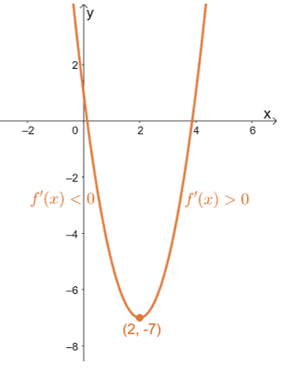 This also confirms how vertices represent a quadratic function’s extremum. Apply the same steps we’ve used to find other function’s extremum. Don’t worry, you’ll be able to use the first derivative test in our example section later! For now, let’s move on to our next derivative test: the second derivative test.
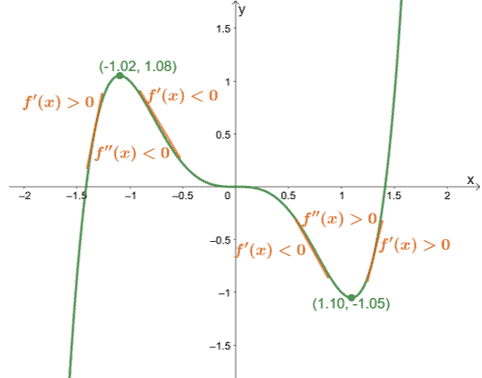 Here’s an example of a function ($f(x) = x^5 -2x^3$) with two local extremums. We can confirm this by observing the signs of $f”(x)$ at these two critical points.