Double Integrals – Definition, Formula, and Examples

The double integral allows us to extend our understanding of areas under the curve from the two-dimensional coordinate system to volumes under the surfaces in a three-dimensional coordinate system. Double integrals allow us to calculate mass densities and estimate probability density functions – just two of the many functions of double integrals!

The double integral allows us to calculate the volume under the space bounded by the region, $\boldsymbol{R}$. We can evaluate double integrals by evaluating integrals with respect to one variable and keeping the rest of the variable constant.

This article covers all the key concepts we need to understand what double integrals represent. By the end of the discussion, we want you to feel confident when solving problems that involve double integrals.

What Is a Double Integral?                 

The double integral represents the integral of the function, $f(x, y)$ over a given region, $R$. Suppose that for a region, $R$, is defined by $x \in [a, b]$ and $y \in [c, d]$, we can define the double integral of the function, $f(x, y)$, in the region ($R$) is given by the expressions below.

\begin{aligned}\int \int_{R} f(x, y) \phantom{dx}dA\\\int_{c}^{d} \int_{b}^{a} f(x, y) \phantom{x}dxdy\end{aligned}

The double integral is also an important example of iterated integrals. Its general form alone highlights this – we integrate the double variable function with respect to one variable then the next. We’ll explore more about the process of evaluating double integrals later, but for now, we’ll need to understand what double integrals represent and how we’ve established its rules.

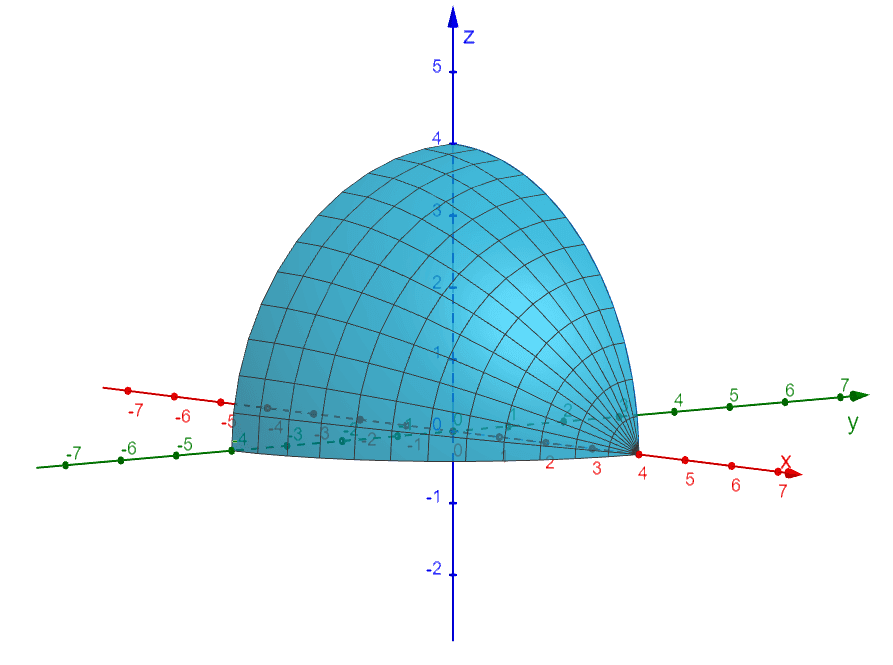
Through double integrals, we can now calculate the surface area of curves like the one shown above and projected at different planes. We begin our understanding of double integrals by reviewing what we know of definite integrals. Recall that through the fundamental theorem of calculus, we can define definite integrals as shown below.

\begin{aligned}\int_{a}^{b} f(x) \phantom{x}dx &= \lim_{n \rightarrow  \infty}[f(x_1)\Delta x + f(x_2)\Delta x + …+ f(x_n)\Delta x]\\\Delta x &= \dfrac{b – a}{n}\end{aligned}          

As we have learned in the past, $\Delta x$ represents the width of the rectangles and $\{x_1, x_2, x_3, …, x_n\}$ are the endpoints formed by the subintervals within the interval, $[a, b]$. Now, how does this relate to double integrals?

Interpreting Double Integrals Using Riemann Sum

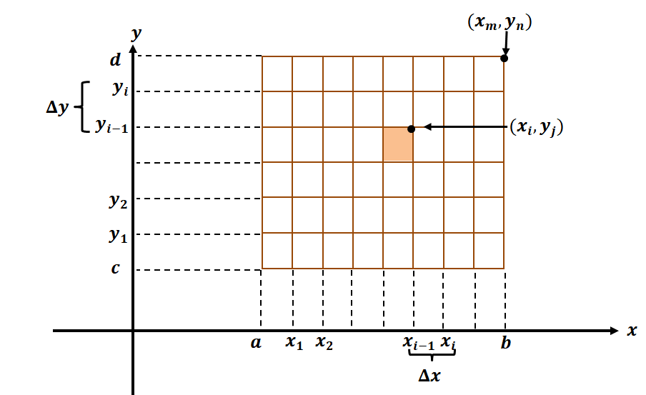
Suppose that we have the region, $R$, bounded by the intervals, $[a, b] \times [c, d]$ across the intervals along the $x$ and $y$-axis, respectively. This means that we can divide the length and width into smaller subintervals and rectangles as shown by the image above. The rectangle contains $mn$ rectangles where each smaller rectangle has an area of $\Delta x \Delta y$, where $\Delta x = \dfrac{b – a}{m}$ and $\Delta y = \dfrac{c – d}{n}$. We can define double integrals in terms of the sum of the areas of the rectangles formed by the graph – similar to how we established the definition for definite integrals before.

Now, let’s extend this understanding by interpreting $f(x_i, y_j)$ as the height of a rectangular prism that has a base area of $A$.

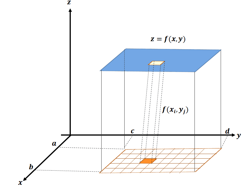
This means that the double integral representing the sum of the rectangular columns will actually represent the volume of the series with a base area bound by the intervals, $[a, b] \times [c, d]$. This is how we define the double integral of the function, $f$, over the rectangular region, $R$.

Hence, the double integral represents the volume found under our surface. This is one way for us to interpret double integrals. Now, let’s view double integrals as iterated integrals.

Interpreting Double Integrals as Iterated Integrals

As we have mentioned earlier, double integrals are essential examples of iterated integrals.

Iterated integrals are integrals of multivariable functions where we evaluate the definite integrals of the function with respect to one variable first then integrate on the next variable. Let’s look back into our expression for the double integral by going back to our function, $f$, defined by two variables and can be integrated within the rectangular region, $R = [a, b] \times [c, d]$. This means that we can integrate $f(x, y)$ with respect to $x$ from $x = a$ to $x = b$ and treat $y$ as a constant.

\begin{aligned}A(y) &= \int_{a}^{b} f(x, y) \phantom{x}dx \end{aligned}

Now, let’s integrate the resulting function, $A(x)$, with respect to $y$ from $y = c$ to $y = d$. This time, we’ll treat $x$ as a constant.

\begin{aligned}\int_{c}^{d} A(y) \phantom{x}dy &=\int_{c}^{d}  \left[\int_{a}^{b} f(x, y) \phantom{x}dx \right] \phantom{x}dy \end{aligned}

Let’s use the original expression for $A(y) = \int_{a}^{b} f(x, y) \phantom{x}dx$ on the left-hand side of the equation.

\begin{aligned}\int_{c}^{d} \int_{a}^{b} f(x, y) \phantom{x}dx \phantom{x}dy &=\int_{c}^{d}  \left[\int_{a}^{b} f(x, y) \phantom{x}dx \right] \phantom{x}dy \end{aligned}

We can rewrite the double integral by integrating $f(x, y)$ with respect to $x$ from $a$ to $b$ then with respect to $y$ from $c$ to $d$.

\begin{aligned}\int_{a}^{b} \int_{c}^{d} f(x, y) \phantom{x}dy \phantom{x}dx &=\int_{a}^{b}  \left[\int_{c}^{d} f(x, y) \phantom{x}dy \right] \phantom{x}dx \end{aligned}

Hence, we‘ve shown how double integrals can be interpreted as iterated integrals. We’ll use this interpretation to solve double integrals in the section shown below.

Interpreting Double Integrals as an Area of General Regions

There are instances when the area of the surface we’re working on does not form a rectangle. Let’s now observe two examples of regions that are not rectangular in shape.

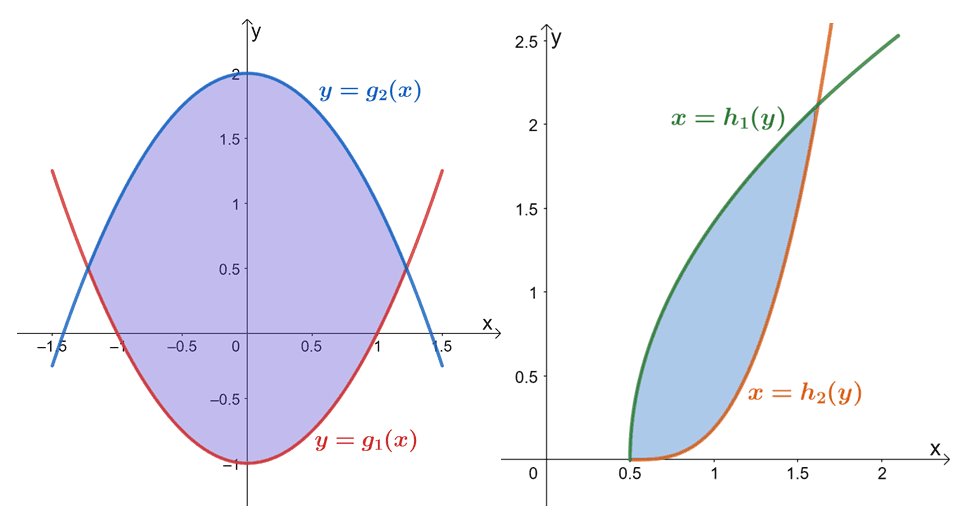
This means that we can now work with surfaces with irregular regions and the two graphs shown above are great examples. The first graph shows a region formed by two curves in terms of $x$ while the second graph shows a region formed by curves in terms of $y$.

\begin{aligned}R &= \{(x, y)| a \leq x \leq b,g_1(x) \leq y \leq g_2(x)\}\\\\R &= \{(x, y)| h_1(y) \leq x \leq h_2(y), c \leq y \leq d\}\end{aligned}

These are the set builder notations that describe the two regions – the first equation describes the region of the leftmost graph and the second set builder notation represents the right graph. We can calculate double integral bounded by the regions shown below.

\begin{aligned}\textbf{Case 1:}\phantom{xxxxxx}\\R = \{(x, y)| a &\leq x \leq b, g_1(x) \leq y \leq g_2(x)\}\\\int \int_R f(x, y) \phantom{x}dA &=\int_{a}^{b} \int_{g_1(x)}^{g_2(x)} f(x, y) dy\phantom{x} dx\\\\\textbf{Case 2:}\phantom{xxxxxx}\\R =\{(x, y)| h_1&(y) \leq x \leq h_2(y), c \leq y \leq d\}\\\int \int_R f(x, y) \phantom{x}dA &=\int_{c}^{d} \int_{h_1(y)}^{h_2(y)} f(x, y) dx\phantom{x} dy\end{aligned}

We’ve shown how to double integrals work for more general regions. Let’s now move on to applying what we’ve learned so far to evaluate double integrals.

How To Solve Double Integrals?               

We can solve problems involving double integrals by applying the appropriate interpretations of double integrals. The fastest way to evaluate double integrals is by using the fact that they are iterated integrals.

• Determine the limits of integration of the function in terms of two variables (normally $x$ and $y$).
• Evaluate the inner integral by working on one variable while treating the other as constant.
• Now, work out the outer integral using the resulting expression.

There are also some properties of double integrals that can help you in evaluating double integrals. Let’s go over some of these properties first!

Properties of double integrals

Given that the functions, $f(x, y)$ and $g(x, y)$, can be integrated throughout the regions, $R$ and $S$, they satisfy the following equations:

1. $\int \int_{R} [f(x, y) \pm g(x, y)]\phantom{x}dA = \int \int_{R} f(x, y) \phantom{x}dA \pm \int \int_{R} g(x, y) \phantom{x}dA$
2. $\int \int_{R} f(x, y) \phantom{x} dA = k \int \int_{R} f(x, y) \phantom{x}dA$, where $k$ is constant
3. When $f(x, y) \leq g(x, y)$ within the region, $R$, the inequality, $\int \int_{R} f(x, y) \phantom{x}dA \leq \int \int_{R} g(x, y) \phantom{x}dA $.
4. If $f(x, y) \geq 0$ within $R$ and the regions $R$ and $S$ are not overlapping each other, then we can write $\int \int_{R \cup S} f(x, y)\phantom{x} dA$ as shown below.

\begin{aligned} \int \int_{R \cup S} f(x, y)\phantom{x} dA  = \int \int_{R} f(x, y) \phantom{x} dA + \int \int_{S} f(x, y) \phantom{x}dA\end{aligned}

Now that you know the different properties of double integrals, it’s time for us to show you an example of solving double integrals.

\begin{aligned}\int_{y = 1}^{4} \int_{x = 0}^{2} 2(1 – xy) \phantom{x}dxdy\end{aligned}

To evaluate the integral shown above, we first factor out $2$ from the double integral. We then integrate the function with respect to $x$ from $x =0$ to $x = 2$ and treat $y$ as if it’s a constant.

\begin{aligned}\int_{y = 1}^{4} \int_{x = 0}^{2} 2(1 – xy) \phantom{x}dxdy &= 2\int_{y = 1}^{4} \left[\int_{x = 0}^{2} (1 – xy) \phantom{x}dx \right ]dy\\&= 2\int_{y = 1}^{4} \left[x – \dfrac{x^2}{2} \cdot y \right ]_{0}^{2} \phantom{x}dy\\&= 2\int_{y = 1}^{4} \left[\left(2- \dfrac{2^2y}{2}\right) – \left(0 – \dfrac{0^2y}{2}\right) \right ]\phantom{x}dy\\&= 2\int_{y = 1}^{4} (2 – 2y) \phantom{x}dy\end{aligned}

We now evaluate the resulting integral with respect to $y$ from $y = 1$ to $y = 4$.

\begin{aligned}\int_{y = 1}^{4} \int_{x = 0}^{2} 2(1 – xy) \phantom{x}dxdy &=2\int_{y = 1}^{4} (2 – 2y)\phantom{x}dy \\&=2\left[2y – 2 \cdot \dfrac{y^2}{2} \right ]_{1}^{4}\\&= 2\left[2y – y^2 \right ]_{1}^{4}\\&= 2[(8 – 16) – (2 – 1)]\\&= -18\end{aligned}

This means that $\int_{y = 1}^{4} \int_{x = 0}^{2} 2(1 – xy) \phantom{x}dxdy$ is equal to $-18$. Getting the hang of it? Don’t worry, we’ve prepared more examples for you! Review the article then test your knowledge with our sample problems shown below.

Example 1

Determine the volume, $V$, found right below the plane, $z = 4x + 2y$ over the rectangular region, $R = [0, 2]\times [0, 4]$.

Solution

Let’s first identify the limits of the double integral: we want to evaluate the double integral of $z = 4x + 2y$ with respect to $x$ from $x = 0$ to $x = 2$. We can then evaluate the expression with respect to $y$ from $y = 0$ to $y = 4$.

\begin{aligned}V &= \int_{y = 0}^{4}\int_{x = 0}^{2} (4x + 2y) \phantom{x}dxdy\end{aligned}

We can factor out $2$ from the double integral then integrate the function with respect to $x$ by treating $2y$ like a constant.

\begin{aligned}V &= \int_{y = 0}^{4} \int_{x = 0}^{2} 2(2x + y) \phantom{x}dxdy\\&= 2\int_{y = 0}^{4} \left[\int_{x = 0}^{2} (2x + y) \phantom{x}dx \right ]dy \\&= 2\int_{y = 0}^{4} \left[2 \cdot \dfrac{x^2}{2} + xy\right ]_{0}^{2} \phantom{x}dy\\&= 2\int_{y = 0}^{4} \left[x^2 + xy\right ]_{0}^{2} \phantom{x}dy\\&= 2\int_{y = 0}^{4} [(2^2 + 2y) – (0^2 + 0)]\phantom{x}dy\\&= 2\int_{y = 0}^{4} (4 + 2y )\phantom{x}dy\end{aligned}

We’re now working with the outer integral, so evaluate the resulting expression with respect to $y$ from $y = 0$ to $y = 4$.

\begin{aligned}V &= 2\int_{y = 0}^{4} (2y + 4)\phantom{x}dy\\&= 2 \left[2 \cdot \dfrac{y^2}{2} + 4y \right ]_{0}^{4}\\&= 2[y^2 + 4y]_{0}^{4}\\&= 2[(4^2 + 4\cdot 4) -(0 + 0)]\\&= 2(32)\\&= 64\end{aligned}

This means that the volume, $V$, under the plane is equal to $64$. Try switching the order of integration and you should be able to come up with the same value!

Example 2   

Determine the volume, $V$, found right below the plane, $z = e^{2x – y}$ over the rectangular region, $R =[1, 4]\times [1, 2]$.

Solution

We have $f(x, y) = e^{2x – y}$ which will always be greater than zero throughout $x$ and $y$. We’re evaluating the double integral so that $x \in [1, 4]$ and $y \in [1, 2]$.

\begin{aligned}V &= \int_{y = 1}^{4} \int_{x =1}^{2} e^{2x – y} \phantom{x}dxdy\end{aligned}

Let’s first integrate the plane with respect to $x$ and treat $y$ as a constant variable. We’ll have to apply the u-substitution method to integrate $\int e^{2x – y} \phantom{x}dx$.

\begin{aligned}u = 2x – y &\Rightarrow du = 2\phantom{x}dx\\\int e^{2x – y} \phantom{x}dx &= \dfrac{1}{2}\int e^u \phantom{x}du\\&= \dfrac{1}{2}e^u\\&= \dfrac{1}{2}e^{2x – y}\end{aligned}

Now, use this expression to evaluate the integral from $x = 1$ to $x = 4$.

\begin{aligned}V &= \int_{y = 1}^{4} \left[\int_{x =1}^{2} e^{2x – y} \phantom{x}dx \right ]dy\\&= \int_{y = 1}^{4} \left[\dfrac{1}{2}e^{2x – y}\right ]_{1}^{2} \phantom{x}dy\\&= \dfrac{1}{2}\int_{y = 1}^{4}\left[e^{2x – y}\right ]_{1}^{2} \phantom{x}dy\\&= \dfrac{1}{2}\int_{y = 1}^{4}\left(e^{4- y} + e^{2 – y}\right) \phantom{x}dy\end{aligned}

Apply a similar process to integrate the outer integral from $y = 1$ to $y = 2$ as shown below.

\begin{aligned}V &= \dfrac{1}{2}\int_{y = 1}^{4}\left(e^{4- y} + e^{2 – y}\right) \phantom{x}dy\\&= \dfrac{1}{2}\left[-e^{4 – y} – e^{2- y}  \right ]_{1}^{4}\\&= \dfrac{1}{2}[(-e^{4 – 4} – e^{2 -4}) – (-e^{4 – 1} – e^{2 -1})]\\&= \dfrac{1}{2}(-e^0 – e^{-2} + e^3 – e)\\&= \dfrac{e^3  – e – 1- e^{-2}}{2}\\&= \dfrac{e^5 – e^{3} – e^2 – 1}{2e^2}\end{aligned}

Hence, we have $V = \dfrac{e^5 – e^{3} – e^2 – 1}{2e^2}$ or approximately equal to $8.25$.

Practice Questions

1. Determine the volume, $V$, found right below the plane, $z = 3x – 6y$ over the rectangular region, $R =[0, 3] \times [0, 1]$.
2. Determine the volume, $V$, found right below the plane, $z = e^{3x + y}$ over the rectangular region, $R =[1, 3]\times [1, 4]$.

Answer Key

1.$ V = \int_{y = 0}^{1}\int_{x = 0}^{3} (3x – 6y) \phantom{x}dxdy = 4.5$
2. $ V = \int_{y = 1}^{4}\int_{x = 1}^{3} e^{3x\:+\:y}\phantom{x}dxdy = \dfrac{e^{13}-e^{10}-e^7+e^4}{3} $

Images/mathematical drawings are created with GeoGebra.