Fundamental Theorem for Line Integrals – Theorem and Examples

The fundamental theorem of line integrals shows us how we can extend the fundamental theorem of calculus when evaluating line integrals.  By generalizing the fundamental theorem of calculus to include line integrals, we can also establish interesting properties about a line integral’s paths. Line integrals are essential in finding potential functions and have extensive applications in physics in engineering, so it’s important that we know easier ways to evaluate line integrals.

The fundamental theorem of line integrals tells us that we can integrate the gradient of a function by evaluating the function at the curves’ endpoints.

In this article, we’ll establish and prove the fundamental theorem of line integrals. We’ll also show you how to apply this in evaluating line integrals. By the end of this discussion, we’ll let you try our different problems so you can further solidify your understanding of this theorem.

What Is the Fundamental Theorem of Line Integrals?

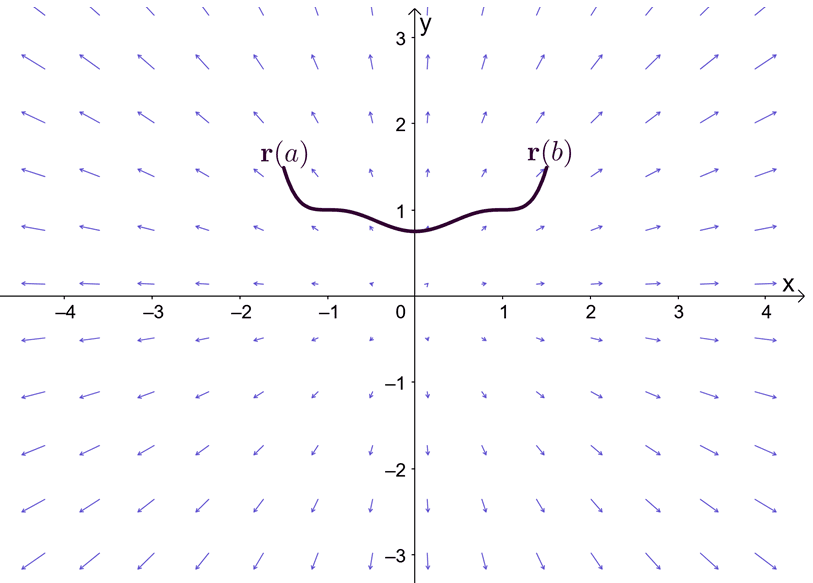
According to the fundamental theorem of line integrals, when we have a curve,$C$, defined by the vector function, $\textbf{r}(t)$, we have the following relationship.

\begin{aligned}\int_{C} \nabla f \cdot d\textbf{r} &= f(\textbf{b}) -f(\textbf{a})\end{aligned}

Keep in mind that the theorem applies when $\textbf{a}= \textbf{r}(a)$ and $\textbf{b}= \textbf{r}(b)$.           

The expression, $\nabla f$, represents the gradient of the function, $f$, and this is why the other name for the fundamental theorem of line integral is the gradient theorem. The graph shows that $\textbf{r}(a)$ and $\textbf{r}(b)$ are the endpoints of the curve.

Before we explore the gradient theorem, let’s do a quick recall of the fundamental theorem for single variable calculus – particularly, the part of the theorem that expounds on definite integrals. Suppose that $F^{\prime}(x) = f(x)$ and $F(x)$ is differentiable throughout the interval, $[a, b]$, we can define the definite integral as shown below.

\begin{aligned} \int_{a}^{b} f^{\prime}(x) \phantom{x}dx &= F(b) – F(a)\end{aligned}  

Now, let’s extend this with gradients, $\nabla f(x, y)$ or $\nabla f(x, y, z)$, to establish the rules for the fundamental theorem of line integrals. We’ll focus on $\nabla f(x, y, z)$ in proving the theorem. Suppose that $\textbf{r}(t) = <x(t), y(t), z(t)>$, we can write $\nabla f(x, y, z) \cdot d\textbf{r}$ as shown below.

\begin{aligned} \nabla f \cdot d\textbf{r} &= \left<\dfrac{\partial f}{\partial x},\dfrac{\partial f}{\partial y}, \dfrac{\partial f}{\partial z}\right> \cdot \left<\dfrac{dx}{dt}, \dfrac{dy}{dt}, \dfrac{dz}{dt}\right>\\&= \left(\dfrac{\partial f}{\partial x} \dfrac{dx}{dt} + \dfrac{\partial f}{\partial y} \dfrac{dy}{dt} + \dfrac{\partial f}{\partial z} \dfrac{dz}{dt}\right ) \phantom{x}dt\end{aligned}

Applying the chain rule will lead to our simplified expression for $\nabla f(x, y, z) \cdot d\textbf{r}$.

\begin{aligned} \nabla f \cdot d\textbf{r} &= \dfrac{d}{dt}f(\textbf{r}(t))\end{aligned}

Take the line integral of both sides of the equation so that the line integral is evaluated at the smooth curve, $C$, where $a \leq t \leq b$.

\begin{aligned}\int_{C} \nabla f \cdot d\textbf{r} &= \int_{a}^{b}\dfrac{d}{dt}f(\textbf{r}(t))\\&= f(\textbf{r}(a) – \textbf{r}(b))\end{aligned}

This confirms the fundamental theorem or gradient theorem for line integrals. From the equation, we can see that the line integral of a $\nabla f$ represents the change of $$ from its endpoints, $\textbf{r}(a)$ and $\textbf{r}(b)$. Now that we’ve established its equation, it’s important that we know when and how to apply this essential theorem.

How To Use the Fundamental Theorem of Line Integrals?

Apply the fundamental theorem of line integrals to shorten the process of evaluating the line integrals along a path. We can do so by doing the following steps:

1. Identify the expression for, $f(x, y)$ or $f(x, y,z)$.If it’s not yet given, use the fact that $\textbf{F} = \nabla f$.
2. If the endpoints are given and the path is not specified, evaluate the line integral by taking the difference between endpoints: $\textbf{r}(b)$ and $\textbf{r}(a)$.
3. When given $f(x,y)$ or $f(x,y,z)$, use this and evaluate the function at $\textbf{r}(a)$ and $\textbf{r}(b)$.
4. Find the difference between the two evaluated endpoints.

This simplifies our process of evaluating line integrals. Let’s evaluate the line integral, $\int_{C} \textbf{F} \cdot d\textbf{r}$, using two methods: 1) using the traditional method of evaluating line integrals and 2) by applying the fundamental theorem of line integrals.

\begin{aligned}\textbf{F}(x, y) &= \nabla f(x,y)\\ f(x,y) &= 2\cos x – x^2y\end{aligned}

We’re evaluating the line integral over the curve, $C$ parametrized by the vector function, $\textbf{r}(t) = <-t, t^2>$, from $0 \leq t \leq \pi$.

Traditionally, we’ll find $\nabla f$ first and evaluate them at the endpoints using $\textbf{r}(t)$. We use the definition of line integrals as shown below.

\begin{aligned}\int_{C} \textbf{F} \cdot d\textbf{r} &= \int_{0}^{\pi} \textbf{F}(\textbf{r}(t)) \cdot \textbf{r}^{\prime}(t) \phantom{x}dt\end{aligned}

Now, recall that $\nabla f(x, y) = \left<\dfrac{\partial f}{\partial x}, \dfrac{\partial f}{\partial y}\right>$, so apply this definition if we want to find $\textbf{F}(x, y)$.

\begin{aligned}\textbf{F}(x, y) &= \left<\dfrac{\partial f}{\partial x}, \dfrac{\partial f}{\partial y}\right>\\&= \left<-2 \sin x – 2xy, -x^2\right>\end{aligned}

Let’s evaluate the gradient of $f(x,y)$ at $\textbf{r}(t) = <-t, t^2>$.

\begin{aligned}\textbf{F}(\textbf{r}(t)) &= \textbf{F}(<-t, t^2>)\\&= \left<-2 \sin (-t) – 2(-t)(t^2), -(-t)^2\right>\\&= \left<2\sin t+ 2t^3, -t^2\right>\end{aligned}

Find the dot product of $\textbf{F}(\textbf{r}(t))$ and $\textbf{r}^{\prime}(t)$ then evaluate the resulting integral.

\begin{aligned}\int_{0}^{\pi} \textbf{F}(\textbf{r}(t)) \cdot \textbf{r}^{\prime}(t) \phantom{x}dt &=\int_{0}^{\pi}\left<2\sin t+ 2t^3, -t^2\right> \cdot<-1, 2t>\phantom{x} dt\\&=\int_{0}^{\pi}(2\sin t + 2t^3)(-1) + (-t^2)(2t) \phantom{x}dt\\&=\int_{0}^{\pi} -2\sin t – 4t^3 \phantom{x}dt \\&= \left[2\cos t – t^4\right ]_{0}^{\pi}\\&= \left(2\cos \pi – \pi^4\right )  -\left(2\cos 0 – 0\right )\\&= -4 – \pi^4\end{aligned}

Now, let us show you how to evaluate the line integral $\int_{C} \textbf{F} \cdot d\textbf{r}$ using the gradient theorem. This time, we’ll evaluate $f(x, y)$ for $\textbf{r}(0)$ and $\textbf{r}(\pi)$ then find their difference to find the line integral’s value.

\begin{aligned}\int_{C} \textbf{F} \cdot d\textbf{r} &= f(\textbf{r}(\pi)) – f(\textbf{r}(0))\\&=f(<-\pi, \pi^2>) -f(<0, 0>)\\&= [(2\cos (-\pi) – (-\pi)^2(\pi^2)) – (2\cos 0 – (0)^2(0))]\\&= (-2- \pi^4) – 2\\&= -4 – \pi^4\end{aligned}

This returns the same value from the one where we applied the traditional approach. As you can see, the steps needed to get to our value are much simpler if we use the fundamental theorem of line integrals.

When To Use Fundamental Theorem of Line Integrals?

We can use the fundamental theorem of line integrals to evaluate integrals faster – we’ve shown to in the past sections. It’s time for us to highlight some important applications of this theorem. We can use the fundamental theorem of line integrals to establish other theorems.

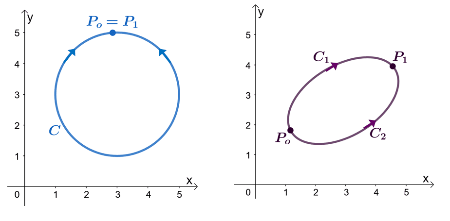
For example, we have the two graphs shown above: the left graph shows a curve with a closed path, and the right graph shows. Suppose that $\textbf{F}$ is a vector field that has components that have partial derivatives. When our line integral is going through a smooth piecewise curve, $C$, we have the following statements:

1. The vector field, $\textbf{F}$, can be shown to be conservative.
2. The line integral, $\int_{C} \textbf{F} \cdot d\textbf{r}$, is independent of path.
3. When we have a line integral, $\int_{C} \textbf{F} \cdot d\textbf{r}$, of independent, the curve, $C$ is a closed path when $\int_{C} \textbf{F} \cdot d\textbf{r} = 0$.

Let’s try to prove that $\int_{C} \textbf{F} \cdot d\textbf{r} = 0$ when $C$ is a closed path.  Recall that we can evaluate line integral of a smooth curve by evaluating the function, $f(x)$, where $\textbf{F} = \nabla f$, where the endpoints are identical.

\begin{aligned}\int_{C} \textbf{F} \cdot d\textbf{r} &= f(P_1) – f(P_o)\\&= f(P_o) – f(P_o)\\&= 0\\&\Rightarrow \textbf{Closed curve}\end{aligned}

This confirms the third statement – showing how the fundamental theorem for line integrals opens a wide range of properties that involve line integrals of vector fields. Now that we’ve learned how to apply the fundamental theorem for line integrals, it’s time for us to explore other examples to better master this topic!

Example 1

The vector fields shown below are known to represent gradient fields, so calculate $\int_{C} \nabla f \cdot d\textbf{r}$.

a. $\textbf{F} = <3x, -2>$ and $C$ represents a quarter circle from $(3, 0)$ to $(0, 3)$
b. $\textbf{F} = \left<\dfrac{\cos y }{x}, -\ln x \sin y\right>$ and $C$ represents a line segment from $(1, 1)$ to $(2, 4)$
c. $\textbf{F} = <6x^2 + 2y^2, 4xy – 3y^2>$ and $C$ represents a curve passing through $(0, 4)$ to $(4, 0)$

Solution

Thanks to the fundamental theorem for line integrals, we can easily evaluate the three line integrals without going through the process of parametrizing the functions. Since $\textbf{F}  = \nabla f$, we can find $\int_{C} F\cdot d\textbf{r} = \int_{C} \nabla f \cdot d\textbf{r}$ by evaluating $f$ at the endpoints of the curve.

For the first item, we have $\textbf{F} = \nabla f = <3x, -2>$, so for this possible, $f(x,y)  = \dfrac{3}{2}x^2 -2y$. Let’s evaluate $f(\textbf{r}(t))$ at the following endpoints: $(3, 0)$ and $(0, 3)$. Subtract the resulting expressions to find the value of the line integral.

\begin{aligned}\int_{C} F\cdot d\textbf{r} &= \int_{C} \nabla f \cdot d\textbf{r}\\&= f(0, 3) – f(3, 0)\\&= \left[\dfrac{3}{2}(0)^2 -2(3) \right ] -\left[\dfrac{3}{2}(3)^2 -2(0) \right ]\\&= -6 + \dfrac{27}{2}\\&= \dfrac{15}{2}\end{aligned}

a. This means that $\int_{C} \nabla f \cdot d\textbf{r} = \dfrac{15}{2}$.

We’ll apply a similar process for the second item – let’s first determine the expression for $f(x,y )$ given that $\textbf{F} = \left<\dfrac{\cos y }{x}, -\ln x \sin y\right>$. Since $\dfrac{d}{dx} \ln x = \dfrac{1}{x}$ and $\dfrac{d}{dy} \cos y = -\sin y$, we have $f(x,y) = \ln x \cos y$. Evaluate $f(x,y)$ at the following endpoints: $(1, 1)$ and $(2, 4)$.

\begin{aligned}\int_{C} F\cdot d\textbf{r} &= \int_{C} \nabla f \cdot d\textbf{r}\\&= f(2, 4) – f(1, 1)\\&= \left[\ln (2) \cos (4)\right ] -\left[\ln (1) \cos (1) \right ]\\&= \ln 2 \cos 4 \\&\approx -0.45\end{aligned}

b. Hence, we’ve shown that $\int_{C} F\cdot d\textbf{r} = \ln 2 \cos 4$.

Let’s now work on the third item and begin by finding the expression for $f(x, y)$ so that $\nabla f= <6x^2 + 2y^2, 4xy – 3y^2>$. Hence, we have $f(x, y) = 2x^3 + 2xy^2 – y^3$. Now, let’s evaluate this function at the endpoints to find the value of the line integral over the curve, $C$.

\begin{aligned}\int_{C} F\cdot d\textbf{r} &= \int_{C} \nabla f \cdot d\textbf{r}\\&= f(4, 0) – f(0, 4)\\&= \left[2(4)^3 + 2(4)(0)^2 – (0)^3\right ] -\left[2(0)^3 + 2(0)(4)^2 – (4)^3\right ]\\&= 128+ 64\\&= 192\end{aligned}

c. This shows that $\int_{C} F\cdot d\textbf{r} = 192$.

Example 2

Evaluate the line integral, $\int_{C} \nabla f \cdot d\textbf{r}$, where $f(x, y) = x^4(2 – y) + 2y$, and $C$ is a curve that is represented by the vector function, $\textbf{r}(t) = \left< 2 – t^2, 6 + t\right>$, where $-1 \leq t \leq 1$.

Solution

We’re now given $f(x, y)$’s expression, so we can evaluate the function’s endpoints to find the line integral of $\textbf{F} = \nabla f$ over the curve, $C$. Find the value of $\textbf{r}(t)$ at $t = -1$ and $t =1$.

This means that we can evaluate $f(x, y)$ from $(1, 5)$ to $(1, 7)$ then take their difference to find the value of $\int_{C} \nabla f \cdot d\textbf{r}$.

\begin{aligned}\int_{C} \nabla f \cdot d\textbf{r}&= f(1, 7) – f(1, 5)\\&= \left[(1)^4(2 – 7) + 2(7)\right ] -\left[(1)^4(2 – 5) + 2(5)\right ]\\&= 9 – 7\\&= 2\end{aligned}

Hence, we have $\int_{C} \nabla f \cdot d\textbf{r}$ is equal to $2$. This item is another example showing how the fundamental theorem for line integrals has simplified the process of evaluating line integrals.

Example 3

Suppose that $\int_{C} \textbf{F} \cdot d\textbf{r}$ is independent of its path, find the value of the line integral if $C$ is a circle represented by the equation, $(x -4 )^2 + (y – 2)^2 =4$ in a clockwise direction.

Solution

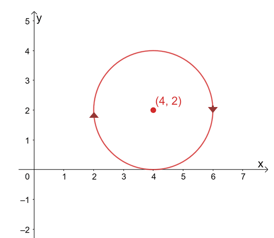
The graph of the curve is a circle centered at $(4, 2)$ and a radius of $2$ units. At a first glance, evaluating the line integral seems like a tedious process, but remember that: 1) $\int_{C} \textbf{F} \cdot d\textbf{r}$ is independent of the path and 2) $C$ is a closed curve representing the entire circle.

\begin{aligned}\int_{C} \textbf{F} \cdot d\textbf{r} &= 0\end{aligned}

Recall that when the line integral is independent of path and defined by a closed curve, its line integral is equal to zero. This also applies to our line integral, hence, it is also equal to zero.

Example 4

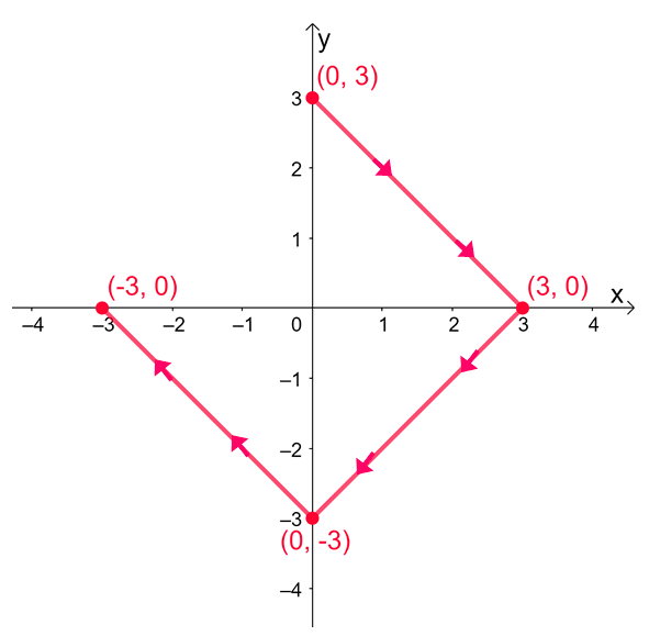
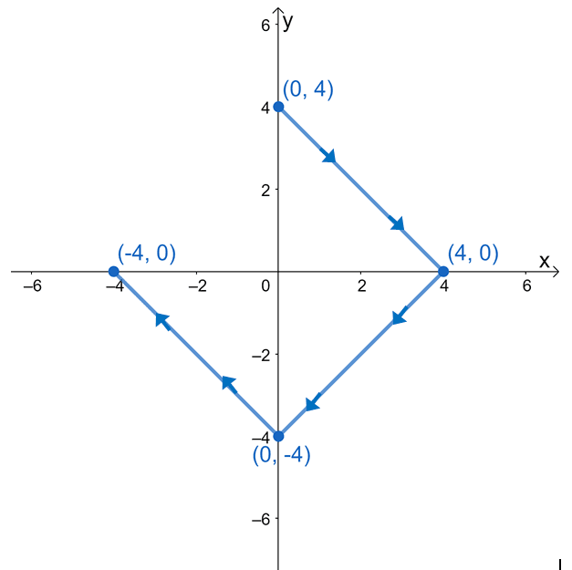
Evaluate the line integral, $\int_{C} \nabla f \cdot d\textbf{r}$, where $f(x, y) = e^{2xy} – 2x^3 + y^4$, and $C$ is a curve defined by the graph shown below.

Solution

It may be tempting for us to evaluate the line integral by breaking down the expressions into three line integrals. Since the curve, $C$, is a smooth curve, we can evaluate the line integral by evaluating $f(x, y)$ at the curve’s endpoints.

\begin{aligned}\int_{C} \textbf{F} \cdot d\textbf{r} &= f(\text{final point}) – f(\text{initial point})\end{aligned}

We have $(0, 3)$ as the initial point and $(-3, 0)$ as the final point. Evaluate these values then take their difference to find the line integral’s value.

This means that $\int_{C} \textbf{F} \cdot d\textbf{r}$ is equal to $-27$.

Example 5

Suppose that the force field is represented by the vector function, $\textbf{F} = <6yz, 6xz, 6xy>$. What is the amount of work done by an object that moves from $(2, 1, 1)$ to $(4, 4, 2)$?

Solution

To find the amount of work done given $\textbf{F}$, we evaluate the line integral, $\int_{C} \textbf{F} \cdot d\textbf{r}$. Since $\textbf{F} = \nabla f$, let’s go ahead and find the expression for $f(x,y, z)$ first.

\begin{aligned}\nabla f(x, y,z) &= <6yz, 6xz, 6xy>\\ f(x, y, z) = 6xyz\end{aligned}

Now, that we have the expression for $f(x, y,z)$, let’s go ahead and evaluate the function at the starting and ending point moved by the object.

\begin{aligned}\textbf{Work} &= \int_{C} \textbf{F} \cdot d\textbf{r} \\&= f(4, 4,2) – f(2, 1, 1)\\&= 6(4)(4)(2) – 6(2)(1)(1)\\&= 192\end{aligned}

Hence, the amount of work done by the object is equal to $192$ units.

Practice Questions

1. The vector fields shown below are known to represent gradient fields, so calculate $\int_{C} \nabla f \cdot d\textbf{r}$.
a. $\textbf{F} = <6x, -4y>$ and $C$ represents a quarter circle from $(1, 0)$ to $(0, 1)$
b. $\textbf{F} = \left<e^xy^2 – 2xy, 2e^xy – x^2\right>$ and $C$ represents a line segment from $(0, 0)$ to $(3, 3)$
c. $\textbf{F} = <6x^2y + 4y, 2x^3 + 4x – 2y>$ and $C$ represents a curve passing through $(0, 2)$ to $(2, 0)$
2. Evaluate the line integral, $\int_{C} \nabla f \cdot d\textbf{r}$, where $f(x, y) = x^3(6 – y) + 4y$, and $C$ is a curve that is represented by the vector function, $\textbf{r}(t) = \left<4 – t^2, 2 – t\right>$, where $-2 \leq t \leq 2$.
3. Suppose that $\int_{C} \textbf{F} \cdot d\textbf{r}$ is independent of its path, find the value of the line integral if $C$ is an ellipse represented by the equation, $\dfrac{(x- 3)^2}{4} + \dfrac{(y -1)^2}{9} = 1$ in a clockwise direction.
4. Evaluate the line integral, $\int_{C} \nabla f \cdot d\textbf{r}$, where $f(x, y) = e^{xy} – 4x^3 + y^2$, and $C$ is a curve defined by the graph shown below.
5. Suppose that the force field is represented by the vector function, $\textbf{F} = <e^y \cos z, x \cos z e^y, -e^y x\sin z>$. What is the amount of work done by an object that moves from $(0, 1,0)$ to $(2, 4, 2\pi)$?

Answer Key

1.
a. $\int_{C} F\cdot d\textbf{r} = -5$
b. $\int_{C} F\cdot d\textbf{r} = 9e^3 – 27$
c. $\int_{C} F\cdot d\textbf{r} = 4$
2. $\int_{C} F\cdot d\textbf{r} = f(0,0) – f(0, 4) = -16$
3. $\int_{C} \textbf{F} \cdot d\textbf{r} = 0$
4. $\int_{C} \nabla f \cdot d\textbf{r} = f(-4, 0) – f(0, 4) = -271$
5. $\textbf{Work} = f(2, 4, 2\pi) – f(0,1, 0) = 2e^4$

Images/mathematical drawings are created with GeoGebra.