Gauss Jordan Elimination – Explanation & Examples

The Gauss-Jordan Elimination method is an algorithm to solve a linear system of equations. We can also use it to find the inverse of an invertible matrix. Let’s see the definition first:

The Gauss Jordan Elimination, or Gaussian Elimination, is an algorithm to solve a system of linear equations by representing it as an augmented matrix, reducing it using row operations, and expressing the system in reduced row-echelon form to find the values of the variables.

In this lesson, we will see the details of Gaussian Elimination and how to solve a system of linear equations using the Gauss-Jordan Elimination method. Examples and practice questions will follow.

What is Gaussian Elimination?

Gaussian Elimination is a structured method of solving a system of linear equations. Thus, it is an algorithm and can easily be programmed to solve a system of linear equations. The main goal of Gauss-Jordan Elimination is:

• to represent a system of linear equations in an augmented matrix form
• then performing the $3$ row operations on it until the reduced row echelon form (RREF) is achieved
• Lastly, we can easily recognize the solutions from the RREF

Let’s see what an augmented matrix form is, the $3$ row operations we can do on a matrix and the reduced row echelon form of a matrix.

Augmented Matrix

A system of linear equations is shown below:

$\begin{array}{rl}2x+3y& =7\\ x–y& =4\end{array}$

We will write the augmented matrix of this system by using the coefficients of the equations and writing it in the style shown below:

$\left[\begin{array}{rrr}2& 3& 7\\ 1& -1& 4\end{array}\right]$

An example using $3$ simultaneous equations is shown below:

$\begin{array}{rl}2x+y+z& =10\\ x+2y+3z& =1\\ –x–y–z& =2\end{array}$

Representing this system as an augmented matrix:

$\left[\begin{array}{rrrr}2& 1& 1& 10\\ 1& 2& 3& 1\\ –1& –1& –1& 2\end{array}\right]$

Row Operations on a Matrix

There are $3$ elementary row operations that we can do on matrices. It won’t change the solution of the system. They are:

1. Interchange $2$ rows
2. Multiply a row by a non-zero ($\ne 0$) scalar
3. Add or subtract the scalar multiple of one row to another row.

Reduced Row-Echelon Form

The Gauss Jordan Elimination’s main purpose is to use the $3$ elementary row operations on an augmented matrix to reduce it into the reduced row echelon form (RREF). A matrix is said to be in reduced row echelon form, also known as row canonical form, if the following $4$ conditions are satisfied:

1. Rows with zero entries (all elements of that row are $0$s) are at the matrix’s bottom.
2. The leading entry (the first non-zero entry in a row) of each non-zero row is to the right of the row’s leading entry directly above it.
3. The leading entry in any non-zero row is $1$.
4. All entries in the column containing the leading entry ($1$) are zeroes.

How to do Gauss Jordan Elimination

There aren’t any definite steps to the Gauss Jordan Elimination Method, but the algorithm below outlines the steps we perform to arrive at the augmented matrix’s reduced row echelon form.

1. Swap rows so that all rows with zero entries are on the bottom of the matrix.
2. Swap rows so that the row with the largest left-most digit is on the top of the matrix.
3. Multiply the top row by a scalar that converts the top row’s leading entry into $1$ (If the leading entry of the top row is $a$, then multiply it by $\frac{1}{a}$ to get $1$ ).
4. Add or subtract multiples of the top row to the other rows so that the entry’s in the column of the top row’s leading entry are all zeroes.
5. Perform Steps $2–4$ for the next leftmost non-zero entry until all the leading entries of each row are $1$.
6. Swap the rows so that the leading entry of each nonzero row is to the right of the leading entry of the row directly above it

At first glance, it’s not that easy to memorize/remember the steps. It’s a matter of solving several problems until you get the hang of the process. There is also the factor of intuition that plays a B-I-G role in performing the Gauss Jordan Elimination.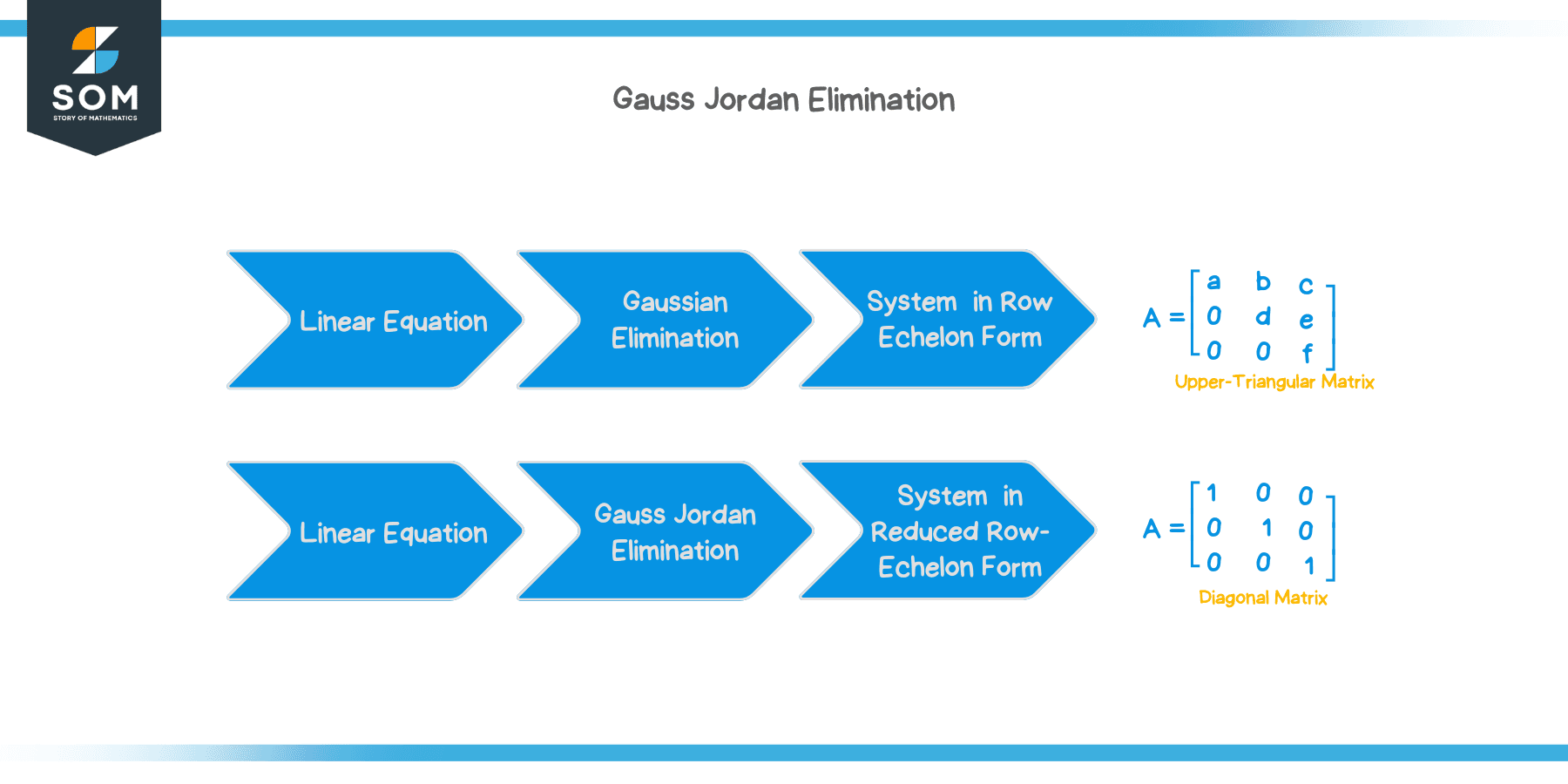

Let’s take a few examples to elucidate the process of solving a system of linear equations via the Gauss Jordan Elimination Method.

Example 1

Solve the system shown below using the Gauss Jordan Elimination method:

$\begin{array}{rl}–x+2y& =–6\\ 3x–4y& =14\end{array}$

Solution

The first step is to write the augmented matrix of the system. We show this below:

$\left[\begin{array}{rrr}–1& 2& –6\\ 3& -4& 14\end{array}\right]$

Now, our task is to reduce the matrix into the reduced row echelon form (RREF) by performing the $3$ elementary row operations.

The augmented matrix that we have is:

$\left[\begin{array}{rrr}–1& 2& –6\\ 3& –4& 14\end{array}\right]$

Step 1:

We can multiply the first row by $–1$ to make the leading entry $1$. Shown below:

$\left[\begin{array}{rrr}1& –2& 6\\ 3& –4& 14\end{array}\right]$

Step 2:

We can now multiply the first row by $3$ and subtract it from the second row. Shown below:

$\left[\begin{array}{rrr}1& -2& 6\\ 3–(1\times 3)& -4–(-2\times 3)& 14–(6\times 3)\end{array}\right]$

$=\left[\begin{array}{rrr}1& –2& 6\\ 0& 2& –4\end{array}\right]$

We have a $0$ as the first entry of the second row.

Step 3:

To make the second entry of the second row $1$, we can multiply the second row by $\frac{1}{2}$. Shown below:

$\left[\begin{array}{rrr}1& –2& 6\\ \frac{1}{2}\times 0& \frac{1}{2}\times 2& \frac{1}{2}\times –4\end{array}\right]$

$=\left[\begin{array}{rrr}1& –2& 6\\ 0& 1& –2\end{array}\right]$

Step 4:

We are almost there! 

The second entry of the first row should be $0$. In order to do that, we multiply the second row by $2$ and add it to the first row. Shown below:

$\left[\begin{array}{rrr}1+(0\times 2)& –2+(1\times 2)& 6+(–2\times 2)\\ 0& 1& –2\end{array}\right]$

$=\left[\begin{array}{rrr}1& 0& 2\\ 0& 1& –2\end{array}\right]$

This is the reduced row echelon form. From the augmented matrix, we can write two equations (solutions):

$\begin{array}{rl}x+0y& =2\\ 0x+y& =-2\end{array}$

$\begin{array}{rl}x& =2\\ y& =–2\end{array}$

Thus, the solution of the system of equations is $x=2$ and $y=–2$.

Example 2

Solve the system shown below using the Gauss Jordan Elimination method:

$\begin{array}{rl}x+2y& =4\\ x–2y& =6\end{array}$

Solution

Let’s write the augmented matrix of the system of equations:

$\left[\begin{array}{rrr}1& 2& 4\\ 1& –2& 6\end{array}\right]$

Now, we do the elementary row operations on this matrix until we arrive in the reduced row echelon form.

Step 1:

We multiply the first row by $1$ and then subtract it from the second row. This is basically subtracting the first row from the second row:

$\left[\begin{array}{rrr}1& 2& 4\\ 1–1& –2–2& 6–4\end{array}\right]$

$=\left[\begin{array}{rrr}1& 2& 4\\ 0& –4& 2\end{array}\right]$

Step 2:

We multiply the second row by $-\frac{1}{4}$ to make the second entry of the row, $1$:

$\left[\begin{array}{rrr}1& 2& 4\\ 0\times -\frac{1}{4}& –4\times -\frac{1}{4}& 2\times -\frac{1}{4}\end{array}\right]$

$=\left[\begin{array}{rrr}1& 2& 4\\ 0& 1& -\frac{1}{2}\end{array}\right]$

Step 3:

Lastly, we multiply the second row by $–2$ and add it to the first row to get the reduced row echelon form of this matrix:

$\left[\begin{array}{rrr}1+(-2\times 0)& 2+(–2\times 1)& 4+(–2\times -\frac{1}{2})\\ 0& 1& -\frac{1}{2}\end{array}\right]$

$=\left[\begin{array}{rrr}1& 0& 5\\ 0& 1& -\frac{1}{2}\end{array}\right]$

This is the reduced row echelon form. From the augmented matrix, we can write two equations (solutions):

$\begin{array}{rl}x+0y& =5\\ 0x+y& =-\frac{1}{2}\end{array}$

$\begin{array}{rl}x& =5\\ y& =-\frac{1}{2}\end{array}$

Thus, the solution of the system of equations is $x=5$ and $y=-\frac{1}{2}$.

Practice Questions

1. Solve the system shown below using the Gauss Jordan Elimination method:

   $\begin{array}{rl}2x+y& =–3\\ –x–y& =2\end{array}$

2. Solve the system shown below using the Gauss Jordan Elimination method:

   $\begin{array}{rl}x+5y& =15\\ –x+5y& =25\end{array}$

Answers

1. We start off by writing the augmented matrix of the system of equations:

   $\left[\begin{array}{rrr}2& 1& –3\\ –1& –1& 2\end{array}\right]$

   Now, we do the elementary row operations to arrive at our solution.

   First,
   We inverse the signs of second row and exchange the rows. So, we have:
   $\left[\begin{array}{rrr}1& 1& –2\\ 2& 1& –3\end{array}\right]$
   Second,
   We subtract twice of first row from second row:
   $\left[\begin{array}{rrr}1& 1& –2\\ 2–(2\times 1)& 1–(2\times 1)& –3–(2\times –2)\end{array}\right]$
   $=\left[\begin{array}{rrr}1& 1& –2\\ 0& –1& 1\end{array}\right]$
   Third,
   We inverse the second row to get:
   $=\left[\begin{array}{rrr}1& 1& –2\\ 0& 1& –1\end{array}\right]$
   Lastly,
   We subtract the second row from the first row and get:
   $=\left[\begin{array}{rrr}1& 0& –1\\ 0& 1& –1\end{array}\right]$

   From this augmented matrix, we can write two equations (solutions):

   $\begin{array}{rl}x+0y& =–1\\ 0x+y& =–1\end{array}$

   $\begin{array}{rl}x& =–1\\ y& =–1\end{array}$

   Thus, the solution of the system of equations is $x=–1$ and $y=–1$.

2. The augmented matrix of the system is:
   $\left[\begin{array}{rrr}1& 5& 15\\ –1& 5& 25\end{array}\right]$
   Let’s  get this matrix to reduced row echelon form and find the solution of the system.
   
   First,
   Negate the first row then subtract it from the second row to get:
   $\left[\begin{array}{rrr}1& 5& 15\\ –1–(–1)& 5–(–5)& 25–(–15)\end{array}\right]$
   $=\left[\begin{array}{rrr}1& 5& 15\\ 0& 10& 40\end{array}\right]$
   Second,
   Divide the second row by $10$ to get:
   $\left[\begin{array}{rrr}1& 5& 15\\ 0& 1& 4\end{array}\right]$
   Then,
   Multiply the second row by $5$ and subtract it from the first row to finally get the solution:
   $\left[\begin{array}{rrr}1–(5\times 0)& 5–(5\times 1)& 15–(5\times 4)\\ 0& 1& 4\end{array}\right]$
   $=\left[\begin{array}{rrr}1& 0& –5\\ 0& 1& 4\end{array}\right]$
   This is the reduced row echelon form (RREF). From this augmented matrix, we can write two equations (solutions):

   $\begin{array}{rl}x& =–5\\ y& =4\end{array}$

   Thus, the solution of the system of equations is $x=–5$ and $y=4$.

Previous Lesson | Main Page | Next Lesson