JUMP TO TOPIC
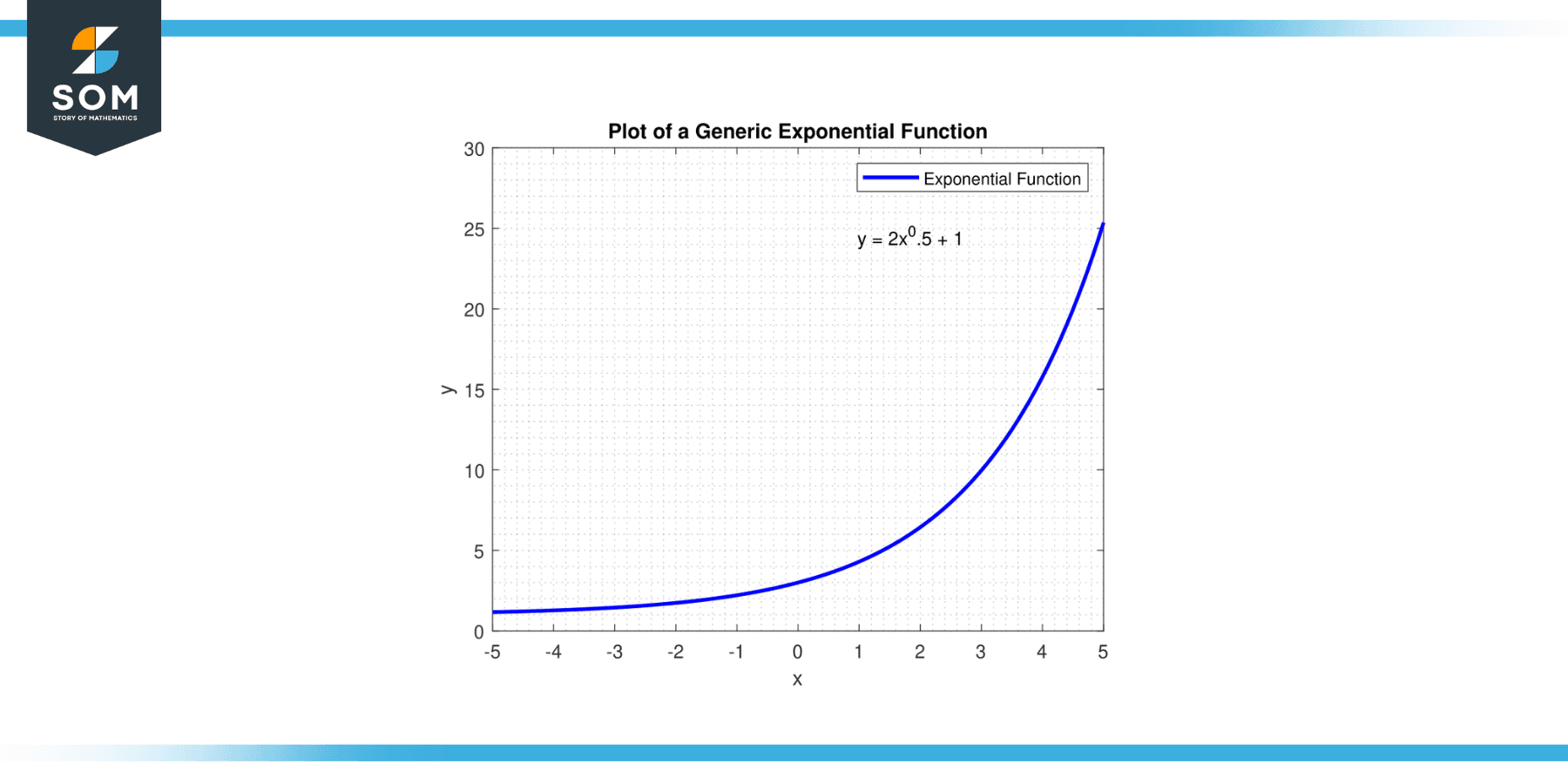
To graph an exponential function, I start by identifying the function’s base, which determines whether the function represents exponential growth or exponential decay.
For example, a function like $y = 5^x$ exhibits growth since the base is greater than 1. I plot points by choosing values for x and calculating the corresponding y values to sketch the curve of the function on a graph.
Exponential functions are vital in various real-world applications, including finance, where they model compound interest, life sciences for population growth, computer science for algorithmic complexity, and forensics for decay processes.
In each case, understanding the direction and shape of the graph helps in predicting future values. If the base of the function is less than 1, then the graph shows decay, representing processes like radioactive decay or depreciation.
To create an accurate representation, I ensure to plot key points such as the y-intercept at $y = b^0$, where b is the base, which always equals 1.
This sets the groundwork for recognizing an exponential function’s signature curve, with one side approaching zero—the horizontal asymptote—and the other rising or falling sharply depending on whether the function models growth or decay. Stay tuned as I show how this dynamic function can bring to light fascinating trends and predictions.
Setting Up the Graph of an Exponential Function
When I’m about to graph an exponential function, my focus is on the behavior of the function, domain and range values, and the graphical characteristics like the horizontal asymptote.

Here’s how I set up the graph of an exponential function, step-by-step.
Creating a Table of Values
Firstly, I like to create a table of values to organize my x and y data points. For a function like $y = b^x$, where b is the base, I choose several x values — positive, negative, and zero. Then I calculate the corresponding y values, which show me the function’s growth or decay.
Table of Values Example:
| x | y |
|---|---|
| -2 | $b^{-2}$ |
| -1 | $ b^{-1}$ |
| 0 | 1 |
| 1 | b |
| 2 | $b^2 $ |
Plotting Points on the Graph
Using the table of values, I plot each pair of x and y coordinates on the graph. This gives me a series of points that, when connected, start to show the characteristic shape of the exponential curve.
Identifying Asymptotes and End Behavior
I also need to determine the horizontal asymptote of the exponential function. For most exponential functions, the horizontal asymptote is the line ( y = 0 ). It’s where the graph approaches but never touches as ( x ) progresses towards negative or positive infinity.
This ties into the end behavior of the function; for a growth function, ( y ) will increase without bound as ( x ) goes to infinity. For decay, the function approaches the horizontal asymptote as ( x ) increases.
Transforming Exponential Graphs
When I graph the exponential functions, I often use various transformations of functions to modify the shape and position of the graph. Understanding these can help anyone tailor the function to fit their data or situation better.
The basic form of an exponential function is $f(x) = b^x$, where $b$ is a positive constant. From this parent function, I can apply different transformations to shift, reflect, stretch, or compress the graph.
Vertical shifts are achieved by adding or subtracting a constant value, which moves the graph up or down. For instance, $f(x) = b^x + k$ would result in a shift up if $k > 0$ and a shift down if $k < 0$.
Horizontal shifts involve adding or subtracting a constant to the input variable, $x$. The function $f(x) = b^{(x-h)}$ represents a shift to the right by $h$ units if $h > 0$ and to the left if $h < 0$.
Reflections are another vital transformation that flips the graph over a specific axis. To reflect a graph across the x-axis, I multiply the function by -1, yielding $f(x) = -b^x$. For a reflection across the y-axis, I would change the sign of the exponent, giving me $f(x) = b^{-x}$.
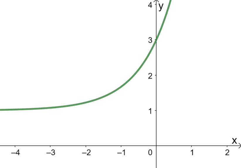
graphing exponential functions 3 1
Lastly, stretches and compressions change the graph’s steepness or width. Multiplying the function by a value $a > 1$ will stretch it vertically, while $0 < a < 1$ will compress it. Similarly, multiplying the exponent by $c > 1$ compresses the graph horizontally, and if $0 < c < 1$, it stretches it.
Here is a quick reference table for these transformations:
| Transformation | Function Form | Effect on Graph |
|---|---|---|
| Vertical Shift | $f(x) = b^x + k$ | Shifts graph up/down by $k$ |
| Horizontal Shift | $f(x) = b^{(x-h)}$ | Shifts graph right/left by $h$ |
| Reflection | $f(x) = -b^x$ | Reflects graph across x-axis |
| $f(x) = b^{-x}$ | Reflects graph across y-axis | |
| Stretch | $f(x) = a \cdot b^x$ | Stretches graph vertically |
| Compression | $f(x) = b^{cx}$ | Compresses graph horizontally |
By applying these transformations systematically, I can shape the graph of an exponential function to fit the data or convey specific information visually. With some practice, these transformations become intuitive, and I can quickly sketch the modified graphs of exponential functions.
Real-World Exponential Models
In my daily encounters, I often come across real-world applications of exponential functions that pique my curiosity. In finance, for instance, the concept is at the heart of understanding compound interest.
Here, the equation to calculate compound interest is $A = P(1 + \frac{r}{n})^{nt}$, where (A) is the amount of money accumulated after (n) years, including interest, (P) is the principal amount, (r) is the annual interest rate, (n) is the number of times that interest is compounded per year, and (t) is the time the money is invested for.
When I turn to forensics, something interesting happens. Exponential equations help me determine the time of death by analyzing the rate of cooling of the human body, which is an application of Newton’s Law of Cooling: $T(t) = T_e + (T_b – T_e)e^{-kt}$.
In computer science, algorithms for certain types of problems, such as sorting algorithms or calculating Fibonacci numbers, can have exponential growth in their runtime, depending on the algorithm’s complexity. This is crucial for making predictions about performance and efficiency.
The life sciences frequently utilize exponential graphs to model population growth or the spread of diseases, which can be dictated by equations like $P(t) = P_0e^{rt}$, where (P(t)) is the population at the time (t), (P_0) is the initial population, (r) is the growth rate, and (t) is time.
Each exponential model starts with a parent function of the form $f(x) = b^x$, which can be tailored to fit specific data and scenarios in the real world. Through analyzing exponential graphs, we can visually grasp the immense impact of exponential growth or decay and better understand the phenomena at hand.
| Field | Exponential Function Example | Purpose |
|---|---|---|
| Finance | $A = P(1 + \frac{r}{n})^{nt}$ | Calculate compound interest |
| Forensics | $T(t) = T_e + (T_b – T_e)e^{-kt}$ | Estimate time of death |
| Computer Science | Algorithm complexity | Predict performance and efficiency |
| Life Sciences | $P(t) = P_0e^{rt}$ | Model population growth or disease spread |
I find that recognizing the power and implications of exponential functions in these areas can be quite insightful and empowering.
Conclusion
I hope my guide on graphing exponential functions has been informative and easy to grasp. When plotting exponential functions such as $y = b^x $, remember to identify a few crucial points. Ideally, you should include the y-intercept $(x=0), (y=1)$ and another point like (x=1), (y=b)) to ensure accuracy in your graph.
Always draw the horizontal asymptote, typically the line (y=0), and recognize its importance in showing the boundary that the function value will never reach.
A smooth curve that connects your plotted points will help visualize the rapid increase or decrease of the function.
Through practice and patience, you’ll find graphing these functions to be straightforward. Keep in mind that the base (b) greatly influences the shape of the curve: if (b > 1), you’re looking at growth, and if (0 < b < 1), it’s a decay.
Understanding how to graph exponential functions is not just about plotting points; it’s about recognizing patterns and behaviors that are fundamental to many natural processes and financial models.
So, next time you see a exponential curve, you’ll appreciate the mathematical beauty and the real-world implications it represents. Keep exploring, and don’t hesitate to revisit the sections on Creating a Table of Points or Understanding Exponential Growth for a refresher.