Lagrange Multipliers – Definition, Optimization Problems, and Examples

The method of Lagrange multipliers allows us to address optimization problems in different fields of applications. This includes physics, economics, and information theory. Seeing the wide range of applications this method opens up for us, it’s important that we understand the process of finding extreme values using Lagrange multipliers.

The Lagrange multiplier represents the constant we can use used to find the extreme values of a function that is subject to one or more constraints.

In this article, we’ll cover all the fundamental definitions of Lagrange multipliers. We’ll also show you how to implement the method to solve optimization problems. Since we’ll need partial derivatives and gradients in our discussion, brush up on your knowledge when you need to. For now, let’s start with understanding how Lagrange multipliers help us solve complex problems!

What Is a Lagrange Multiplier?

Lagrange multipliers equip us with another method to solve optimization problems with constraints. By the end of this article, you’ll appreciate the importance of the following set of equations, where $\boldsymbol{\lambda}$ represents the Lagrange multipliers:

In the past, we’ve learned how to solve optimization problems involving single or multiple variables. These techniques, however, are limited to addressing problems with more constraints. This is when Lagrange multipliers come in handy – a more helpful method (developed by Joseph-Louis Lagrange) allows us to address the limitations of other optimization methods.

The best way to appreciate this method is by illustrating a situation where Lagrange multipliers are most helpful. Let’s say we have a profit function, $f(x, y) = 36x + 72y -x^2 – 2xy – 6y^2$, that predicts the profit earned by a manufacturer of soap bars. In the profit function, $x$ defines the number of soap bars sold per month and $y$ represents the number of hours (per month) spent in marketing.    

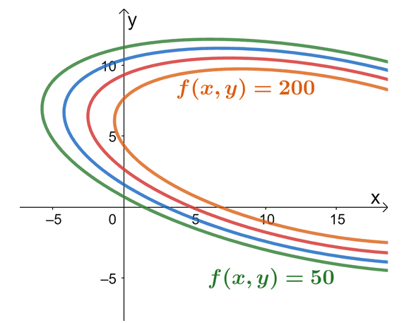
Through our previous knowledge, we’ll be able to calculate the maximum profit per month given a limit on the number of soap bars manufactured per month and a cap on hours spent on marketing. The graph above shows how the objective function, $f(x, y)$, behaves at different constraints: $c = 50, 100, 150,$ and $200$.

Now, what if we make it more interesting by adding a combined constraint on the budget? Suppose that the accounting team wants a budget involving both soap bar production and marketing cost in one inequality: $20x + 4y \leq 120$. The goal remains the same: we want to find the maximum profit possible but for this type, we work with a more complicated constraint. This type of optimization problem is a good example of a situation where we’ll need Lagrange multipliers to address this problem.

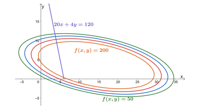
This graph highlights at the values of $f(x,y)$ at different levels of constraint while at the same time, we account for the constraint function, $20x + 4y = 120$. This graph highlights how the variables interact with each of the variables. As we can see from the graph, the farther to the right the graph of $f(x, y)$ is, the smaller the profit. For us to also meet the budget constraint, the ideal profit curve occurs at the point where the constraint function ($20x + 4y = 120$) and the objection function ($f(x, y) = 36x + 72y -x^2 – 2xy – 6y^2$) are tangent to each other. From inspection, we can see it’s somewhere when $c = 200$. Of course, we’ll have a more accurate value once we use the Lagrange multipliers.

The method of Lagrange multipliers simply allows us to find the point where the objective function’s curve is tangent to the constraint function. We’ve learned in the past that a multivariable function’s gradient represents a vector with components that contains two or more variables. When working with vectors, two vectors are lying along the same direction when they share a common factor. This also means that the gradients of both the objective and constraint functions will lie in the same direction. This is where Lagrange multipliers come in.

We can also extend this method to apply them to problems with two or more constraints. Here’s a summary of how the method of Lagrange multipliers can be applied for optimization problems with more than one constraint.

Before we learn how to apply these important conditions to solve optimization problems, let’s see how this formula was established. If you’re too excited to try out problems involving Lagrange multipliers, feel free to head over the next section as well!

Proof of the Lagrange Multiplier Formula

We begin by assuming that $g(x_o, y_o)$ represents the extremum and that the constraint function, $g(x, y) = 0$, is smoothly parametrized by the equations below.

\begin{aligned}x &= x(t)\\ y&= y(t)\end{aligned}

The variable, $t$, represents the parametric arc length with respect to the reference point, $(x_o, y_o)$, at the parameter, $t = 0$. This means that the value of, $z = f(x(t), y(t))$, is a local extremum at $t = 0$. Hence, the derivative of $z$ with respect to $z$ will also be equal to $0$. Writing down the expression for $\dfrac{dz}{dt}$ and applying the chain rule, we have the following equations:

\begin{aligned}\dfrac{dz}{dt} &= \dfrac{\partial f}{\partial x} \cdot \dfrac{\partial f}{\partial t} + \dfrac{\partial f}{\partial y} \cdot \dfrac{\partial y}{\partial t}\\&= \left<\dfrac{\partial f}{\partial x} + \dfrac{\partial f}{\partial y}\right> \cdot \left<\dfrac{\partial x}{\partial t} + \dfrac{\partial y}{\partial t}\right>\\&= 0\end{aligned}

Notice something about $\left<\dfrac{\partial f}{\partial x} + \dfrac{\partial f}{\partial y}\right>$ and $\left<\dfrac{\partial x}{\partial t} + \dfrac{\partial y}{\partial t}\right>$?

• The vector, $\left<\dfrac{\partial f}{\partial x} + \dfrac{\partial f}{\partial y}\right>$, contains the components of $f(x, y)$’s partial derivatives, so this represents the function’s gradient.
• The vector, $\left<\dfrac{\partial x}{\partial t} + \dfrac{\partial y}{\partial t}\right>$, represents the unit tangent vector of the constraint curve.

Using the fact that the point $(x_o, y_o)$ lies in the equation, $t = 0$. We have the following equation as shown below.

\begin{aligned} \nabla f(x_o, y_o) \cdot \textbf{T}(0) &= \end{aligned}

By inspecting the equation, we can see that for the equation to be true, the gradient of $f$ may either represent a zero vector or the normal to the curve constrained at a given local maximum or minimum. This means that when $g(x, y) = 0$ and $\nabla g(x_o, y_o) \neq 0$ is normal to the constraint curve at the point, $(x_o, y_o)$. This confirms the equation,

\begin{aligned}\nabla f(x_o, y_o) &= \nabla g(x_o, y_o),\end{aligned}

where $\lambda$ represents the scalar factor we call the Lagrange multiplier. We can use a similar approach to prove the method for the Lagrange multiplier with two constraints. But we’ll leave that for you to try on your own. Let’s move on to seeing how we can use these conditions to solve different types of optimization problems!

How To Use Lagrange Multipliers?

We can use the Lagrange multipliers to solve problems that involve finding the local minimum or maximum values given one or more constraints. Here are some pointers to remember when working with problems that will benefit from Lagrange multipliers:

• Identify which of the functions represent the objective function, $f(x, y)$, and the constraint function, $g(x, y)$.
• Set up the system of equations associated with one constraint (or two constraints).

• Find the gradients of the functions – take the partial derivatives of each function then write the result as a vector.
• Solve the resulting system of equations to find the values of the variables and the Lagrange multipliers.
• For each of the resulting solutions, calculate the value of $f(x_o, y_o)$ or $f(x_o, y_o, z_o)$ then compare these values.
• Review the problem to determine you’re looking for the maximum or minimum value.

Let’s try to apply these pointers to find the maximum and minimum values of the function,

\begin{aligned} f(x, y) &= 4x + y, \end{aligned}

where this function is subjected to the constraint, $x^2 + y^2 = 12$.  For this problem, it’s easy for us to identify the objective and constraint functions:

• The objective function is equal to $f(x, y) = 4x + y$.
• The constraint function is equal to $g(x, y) = x^2 + y^2 = 12$ or $g(x, y) = x^2 + y^2 – 12 = 0$.

Now that we’ve determined $f(x,y)$ and $g(x,y )$’ expressions, let’s take each of the gradients.

We now have the gradients of the two functions, so we can now set up the system of equations that involve Lagrange multipliers.

\begin{aligned}\nabla f(x_o, y_o) &= \lambda \nabla g(x_o, y_o)\\g(x_o, y_o) &= 0\\& \Downarrow\\ \left<4, 1\right> &= \lambda \left<2x, 2y\right> \end{aligned}

Equate each corresponding component and use $x^2 + y^2 =12$ to have three equations with three variables:

\begin{aligned} 4 &= 2\lambda x \\ 1 &= 2\lambda y\\x^2 + y^2 &= 12\end{aligned}

Substitute $x = \dfrac{2}{\lambda}$ and $y = \dfrac{1}{2\lambda}$ into the third equation  to find the values of the Lagrange multipliers.

\begin{aligned} x^2 + y^2 &= 12\\ \left(\dfrac{2}{\lambda} \right )^2 + \left(\dfrac{1}{2\lambda} \right )^2 &= 12\\ \dfrac{4}{\lambda^2} + \dfrac{1}{4\lambda^2} &= 12\\ 16 + 1 &= 48 \lambda^2\\ \lambda^2 &= \dfrac{17}{48}\\\lambda &= \pm \sqrt{\dfrac{17}{48}}\end{aligned}

Now, substitute these Lagrange multipliers back into our equations for $x$ and $y$ in terms of $\lambda$.

This means that we have the following extreme points: $\left(\dfrac{8\sqrt{3}}{\sqrt{17}}, \dfrac{2\sqrt{3}}{\sqrt{17}}\right)$ and $\left(-\dfrac{8\sqrt{3}}{\sqrt{17}}, -\dfrac{2\sqrt{3}}{\sqrt{17}}\right)$. Now, plug these values into $f(x, y)$ to see which of these two points return the maximum value and the minimum value.

From this, we can see that the maximum value of the function is $2\sqrt{51}$ and occurs at $\left(\dfrac{8\sqrt{3}}{\sqrt{17}}, \dfrac{2\sqrt{3}}{\sqrt{17}}\right)$. Similarly, the minimum value of $f(x, y)$ is $-2\sqrt{51}$ and this happens when $(x, y) = \left(\dfrac{8\sqrt{3}}{\sqrt{17}}, \dfrac{2\sqrt{3}}{\sqrt{17}}\right)$.

Use a similar process when solving optimization problems that involve Lagrange multipliers. Don’t worry, we’ve prepared a wide range of problems for you to work on. When you’re ready, head over to the next two sections to test your understanding and for you to master this topic!

Example 1

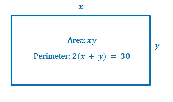
Using the method of Lagrange multipliers, find the dimensions of the rectangle that will maximize its area given that it has a perimeter of $30$ meters.

Solution

Here’s an illustration showing the problem we need to solve: we want to maximize the area, $f(x,y) = xy$, with a constraint of $g(x, y) = 2(x + y) = 30$ or $g(x, y) = 2x + 2y – 30 = 0$.

Now that we’ve identified the objective and constraint functions, let’s write down each of their gradients as shown below.

Let’s now set up the system of equations using the resulting gradients as shown below.

\begin{aligned}\nabla f(x_o, y_o) &= \lambda \nabla g(x_o, y_o)\\g(x_o, y_o) &= 0\\& \Downarrow\\ \left &= \lambda \left<2, 2\right> \end{aligned}

From this, we can see that we can optimize the function when $2x  = \lambda = 2y $ or when $x = \dfrac{\lambda}{2} = y$. Solve the second equation, $2x + 2y – 30 = 0$, and rewrite it using the fact that $x= y$.

\begin{aligned}2x + 2y – 30 &= 0 \\ 2x + 2x – 30&= 0\\4x&= 30\\ x&=  7.5\end{aligned}

This means that we can optimize the value of $f(x, y)$ when $x = y = 7.5$ meters. Since the minimum area occurs when either $x$ or $y$ is equal to zero, our resulting values will return the maximum area of the function.

\begin{aligned}A_{\text{max}} &= (7.5)(7.5)\\&= 56.25\end{aligned}

The maximum area of a rectangle with a perimeter of $30$ meters is equal to $56.25$ squared meters.

Example 2

Now that we know how to use Lagrange multipliers to solve the problem in the first section, why don’t we calculate the maximum profit earned by the soap manufacturer? Here are the following functions discussed earlier:

• The profit earned by the soap bar manufacturer can be modeled by the function, $f(x, y) = 36x + 72y -x^2 – 2xy – 6y^2$, measured in thousands of dollars.
• The accounting team wants to constrain the budget of the number of bars manufactured ($x$) and the number of hours spent in marketing ($y$) with the following function: $g(x, y) = 20x + 4y = 120$.

Estimate the maximum profit to the nearest cents.

Solution

As we have identified earlier, we have the following objective function and constraint function:

\begin{aligned}f(x, y) &= 36x + 72y -x^2 – 2xy – 6y^2\\g(x, y) &= 20x + 4y – 120 = 0\end{aligned}

Take the partial derivatives of the two functions to write down their respective gradients.

Use these gradients to set up a key system of equations we can use to solve for $\lambda$.

\begin{aligned}\nabla f(x_o, y_o) &= \lambda \nabla g(x_o, y_o)\\g(x_o, y_o) &= 0\\& \Downarrow\\ \left<36 - 2x - 2y, 72 - 2x - 12y\right> &= \lambda \left<20,4\right> \end{aligned}

Let’s now break down the equations that we have by equating each component from the left-hand side to the corresponding component from the right-hand side vector. We’ll also use the equation derived from the constraint function, $g(x,y )$.

\begin{aligned}36 – 2x – 2y&= 20\lambda \phantom{x}(1) \\72 – 2x – 12y &= 4\lambda \phantom{xx}(2)\\20x + 4y – 120 &= 0 \phantom{xxx}(3)\end{aligned}

Since $20 \lambda =5 (4\lambda)$, rewrite equation (1) by replacing $20 \lambda$ with four times the expression on the right-hand side of equation (2).

\begin{aligned}72 – 2x – 12y &= 4\lambda\\ 5(72 – 2x – 12y )&= 20\lambda\\&\Downarrow\\36 – 2x – 2y&= 20\lambda\\36 – 2x – 2y&= 5(72 – 2x – 12y )\end{aligned}

With this new equation, let’s find an expression for $x$ in terms of $y$.                   

\begin{aligned}36 – 2x – 2y&= 360 – 10x – 60y\\-2x + 10x &= 360 – 60y + 2y – 36\\8x &= -58y + 324\\ x &= – \dfrac{58}{8}y + \dfrac{324}{8}\\x&= -7.25y + 40.5\end{aligned}

Let’s now use the third equation, $20x + 4y – 120 = 0 $, and the expression of $x$ in terms of $y$.

\begin{aligned}20x + 4y – 120 &= 0 \\20(-7.25y + 40.5) + 4y – 120 &= 0\\-145y + 4y + 810 – 120 &= 0\\-141y &= -690\\y&= \dfrac{690}{141}\\&= \dfrac{230}{47}\\& \approx 4.89\\\\x&= -7.25\cdot \dfrac{230}{47} + 40.5\\&= \dfrac{236}{47}\\&= \approx 5.02\end{aligned}

Now that we have the extremum, $\left(\dfrac{236}{47}, \dfrac{230}{47}\right)$ or $(5.02, 4.89)$, let’s use this to find the maximum profit earned by the manufacturer given the budget constraint.

\begin{aligned}f\left(\dfrac{236}{47}, \dfrac{230}{47}\right) &= 36\left(\dfrac{236}{47}\right) + 72\left(\dfrac{230}{47}\right) -\left(\dfrac{236}{47}\right)^2 – 2\left(\dfrac{236}{47}\right)\left(\dfrac{230}{47}\right) – 6\left(\dfrac{230}{47}\right)^2\\&= \dfrac{14808}{47} \\&\approx 315.06\end{aligned}

This means that the maximum profit earned by the manufacturer is approximately equal to $315. 06$ thousands of dollars (given the budget constraints).

Example 3

Find the maximum and minimum values of the function,

\begin{aligned} f(x, y, z) &= x^2 + y^2 + z^2, \end{aligned}

where this function is subjected to the constraint, $x^3 + y^3 + z^3 = 1 $.                                                            

Solution

We’re now working with three-variable functions with one constraint.

• The objective function is equal to $ f(x, y, z) = x^2 + y^2 + z^2$.
• The constraint function is equal to $g(x, y, z) = x^3 + y^3 + z^3 = 1 $ or $g(x, y, z) = x^3 + y^3 + z^3 – 1= 0$.

As with the previous examples, we’ll evaluate the gradients of the two functions.

Let’s now set up the equation using these two gradients.

\begin{aligned}\nabla f(x_o, y_o, z_o) &= \lambda \nabla g(x_o, y_o, z_o)\\g(x_o, y_o, z_o) &= 0\\& \Downarrow\\ \left<2x, 2y, 2z\right> &= \lambda \left<3x^2, 3y^2, 3z^2\right> \end{aligned}

Using the constraint function and the components of the two vectors, we’ll have the following four equations.

\begin{aligned}2x &= 3\lambda x^2\\2y &= 3\lambda y^2\\2z &= 3\lambda z^2\\ x^3 + y^3 + z^3 &= 1  \end{aligned}

Simplify the first three equations and use their simplified forms to rewrite the fourth equation and solve for $\lambda$.

\begin{aligned}1 &= \dfrac{3}{2}\lambda x\phantom{x}\Rightarrow x = \dfrac{2}{3\lambda}\\ 1 &= \dfrac{3}{2}\lambda y\phantom{x}\Rightarrow y = \dfrac{2}{3\lambda}\\1 &= \dfrac{3}{2}\lambda z\phantom{x}\Rightarrow z = \dfrac{2}{3\lambda}\end{aligned}

\begin{aligned}\left(\dfrac{2}{3\lambda} \right )^3 + \left(\dfrac{2}{3\lambda} \right )^3+ \left(\dfrac{2}{3\lambda} \right )^3 &= 1\\3\left(\dfrac{2}{3\lambda} \right )^3 &= 1\\3\left(\dfrac{8}{27\lambda^3}\right) &= 1\\\lambda^3&= \dfrac{8}{9}\\\lambda &= \sqrt[3]{\dfrac{8}{9}}\end{aligned}

Let’s now plug this value of $\sqrt[3]{\dfrac{8}{9}}$ back into the expressions for $x$, $y$, and $z$.

\begin{aligned} x &= \dfrac{2}{3 \sqrt[3]{\dfrac{8}{9}}}\\&\approx 0.69\\  y &= \dfrac{2}{3 \sqrt[3]{\dfrac{8}{9}}}\\&\approx 0.69\\z &= \dfrac{2}{3\sqrt[3]{\dfrac{8}{9}}}\\&\approx 0.69\end{aligned}

We now have one extreme point to observe, so use these values to find the value of $f(x, y, z)$.

\begin{aligned}f\left(x, y, z\right) &= \left(\sqrt[3]{\dfrac{8}{9}} \right )^2 +\left(\sqrt[3]{\dfrac{8}{9}} \right )^2+\left(\sqrt[3]{\dfrac{8}{9}} \right )^2\\&=\dfrac{4}{\sqrt[3]{3}}\\&\approx 2.77\end{aligned}

To determine whether this represents the local maximum or minimum, let’s see what happens when $x= 0$, $y =0$, or $z= 0$.

This shows that we have a local minimum at $f(x, y,z) = 1$ and a local maximum at $f(x, y,z ) = \dfrac{4}{\sqrt[3]{3}} \approx 2.77$.

Example 4

Determine the points on the circle, $x^2 + y^2 = 64$, that are nearest and farthest from the point, $(-1, 1)$.

Solution

Let’s first write an expression for the distance of the point, $(-1, 1)$, from the circle using the distance formula, $d = \sqrt{(x – x_o)^2 + (y- y_o)^2}$.

\begin{aligned} d &= \sqrt{(x – – 1)^2 + (y-  1)^2}\\&= \sqrt{(x + 1)^2 + (y – 1)^2}\end{aligned}

Keep in mind that if we want to maximize the distance, we’ll also want the square of the distance to be optimized.

\begin{aligned} f(x, y) &= (x + 1)^2 + (y – 1)^2 \end{aligned}

This means that we want to maximize $f(x,y ) (x + 1)^2 + (y – 1)^2 $ constrained to the function, $g(x, y) = x^2 + y^2 = 64$ or $g(x, y) = x^2 + y^2 – 64 = 0$.

Let’s now find the gradients of the two functions as shown below.

Now that we have the gradients of the two functions, set up the system of equations we need to find the values of $x$ and $y$.

\begin{aligned}\nabla f(x_o, y_o) &= \lambda \nabla g(x_o, y_o)\\g(x_o, y_o) &= 0\\& \Downarrow\\ \left<2(x + 1), 2(y -1)\right>  &= \lambda \left<2x, 2y\right> \end{aligned}

This means that we have the following equations from the gradients:

\begin{aligned}2(x + 1) &= 2\lambda x\\ 2(y- 1)&= 2\lambda y\\\dfrac{x – 1}{x} = \lambda &= \dfrac{y -1}{y }\end{aligned}

Now, let’s further simplify this equation as shown below.

\begin{aligned}\dfrac{x – 1}{x} &= \dfrac{y -1}{y }\\xy – y &= xy – x\\ x- y&= 0\\x &= y\end{aligned}

Use $x = y$ into the constraint, $x^2 + y^2 = 64$ to find the value of $x$ and $y$.

\begin{aligned}x^2 + x^2 &= 64\\2x^2 &= 64\\x^2 &= 32\\x&= \pm \sqrt{32}\\x&= \pm 4\sqrt{2}\\\Rightarrow y &=\pm 4\sqrt{2}\end{aligned}

Let’s evaluate the function, $f(x, y)$, at these four critical points to determine which of the four return the maximum and minimum values for $f(x, y)$.

This means that the maximum value of the function is approximately equal to $88.63$ and the minimum value is approximately equal to $43.37$. Hence, the point that is closest to the circle is $(-4\sqrt{2}, 4\sqrt{2})$ while the farthest is $(4\sqrt{2}, -4\sqrt{2})$.

Practice Questions

1. Find the maximum and minimum values of the function,
\begin{aligned} f(x, y) &= 2x – y, \end{aligned}
where this function is subjected to the constraint, $x^2 + y^2 = 4$.

2. Using the method of Lagrange multipliers, find the dimensions of the rectangle that will maximize its area given that it has a perimeter of $40$ feet.

3. Sophie’s company supplies phone cases and she has developed a profit model that depends on the number ($x$) of phone cases supplied per month and the number of hours ($y$) per month allotted for marketing. Here’s the equation for the profit model:
\begin{aligned}z = f(x, y) = 40x + 120y –x^2 – 2xy – 8y^2,\end{aligned}
where $z$ is measured in thousands of dollars. Sophie’s accounting team is proposing a budget constraint modelled by the function, $16x + 4y = 160$.
What are the values of $x$ and $y$ that will return the maximum profit? What is the maximum profit?
4. Find the maximum and minimum values of the function,
\begin{aligned} f(x, y, z) &= x^2 + y^2 + z^2, \end{aligned}
where this function is subjected to the constraint, $x^4 + y^4 + z^4 = 1 $.
5. Determine the points on the circle, $x^2 + y^2 = 80$, that are nearest and farthest from the point, $(1, 2)$.

Answer Key

1. Minimum value: $-2\sqrt{5}$ and maximum value: $2\sqrt{5}$
2. The maximum area is equal to $100$ squared feet.
3. $(x, y) = \left(\dfrac{1020}{121}, \dfrac{760}{121}\right) \approx (8.43, 6.28)$; Maximum profit: $\dfrac{72400}{121} \approx 598.35$ thousands of dollars.
4. Local minimum: $1$ and local maximum: $\sqrt{3} \approx 1.73$
5. Farthest: $(-4, -8)$ and closest: $(1,2)$

Images/mathematical drawings are created with GeoGebra.