JUMP TO TOPIC
Normal Distribution – Explanation & Examples
 The definition of the normal distribution is:
“The normal distribution is a continuous probability distribution that describes the probability of a continuous random variable.”
In this topic, we will discuss the normal distribution from the following aspects:
- What is the normal distribution?
- Normal distribution curve.
- The 68-95-99.7% rule.
- When to use normal distribution?
- Normal distribution formula.
- How to calculate the Normal distribution?
- Practice questions.
- Answer key.
What is the normal distribution?
Continuous random variables take an infinite number of possible values within a certain range.
For example, a certain weight can be 70.5 kg. Still, with increasing balance accuracy, we can have a value of 70.5321458 kg. The weight can take infinite values with infinite decimal places.
Since there is an infinite number of values in any interval, it is not meaningful to talk about the probability that the random variable will take on a specific value. Instead, the probability that a continuous random variable will lie within a given interval is considered.
The probability distribution describes how the probabilities are distributed over the different values of the random variable.
For the continuous random variable, the probability distribution is called the probability density function.
An example of the probability density function is the following:
f(x)={■(0.011&”if ” 41≤x≤131@0&”if ” x<41,x>131)┤
This is an example of uniform distribution. The density of the random variable for values between 41 and 131 is constant and equals 0.011.
We can plot this density function as follows:
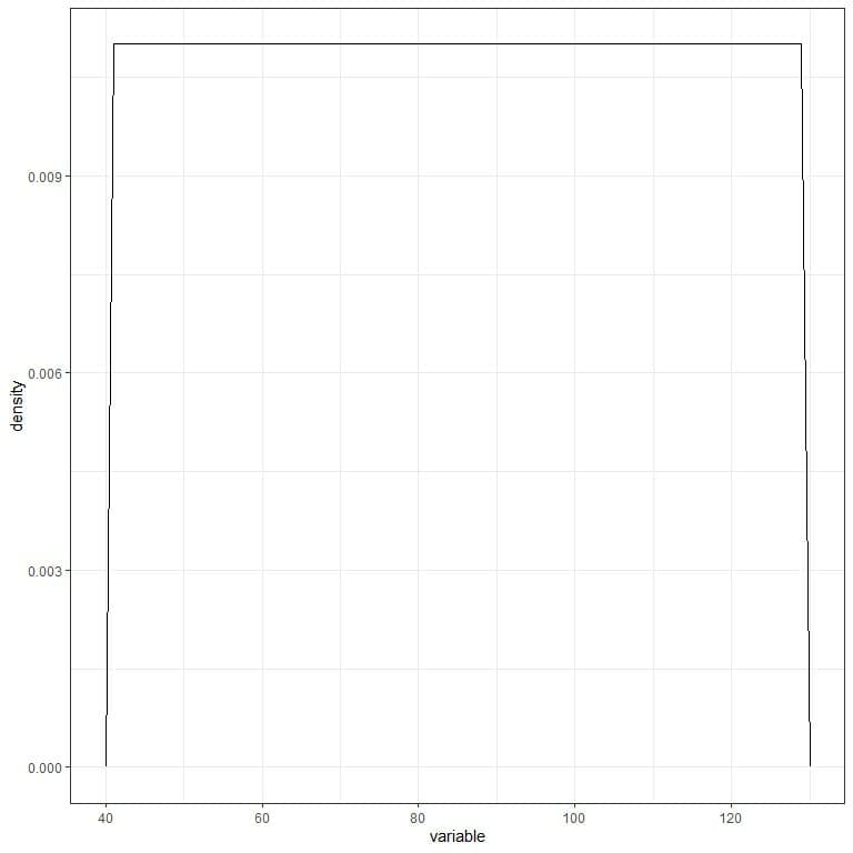
To get the probability from a probability density function, we need to integrate the density (or the area under the curve) for a certain interval.
In any probability distribution, the probabilities must be >= 0 and sum to 1, so the integration of the whole density (or whole area under the curve (AUC)) is 1.
Another example of the probability density function for the continuous random variables is the normal distribution.
The normal distribution is also called the Bell-curve or the Gaussian distribution after the German mathematician Carl Friedrich Gauss discovered it. The face of Carl Friedrich Gauss and the normal distribution curve was on the old German Mark currency.
Characters of the normal distribution:
- Bell-shaped distribution and symmetric around its mean.
- The mean=median=mode, and the mean is the most frequent data value.
- Values closer to the mean are more frequent than values far from the mean.
- The limits of the normal distribution are from negative infinity to positive infinity.
- Any normal distribution is entirely defined by its mean and standard deviation.
The following plot shows different normal distributions with different means and different standard deviations.
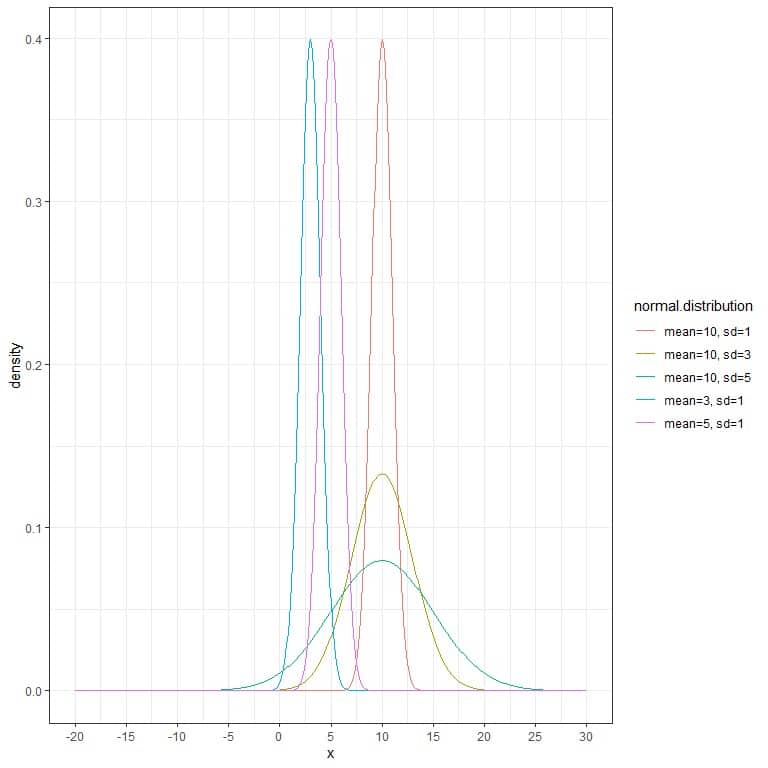
We see that:
- Each normal distribution curve is bell-shaped, peaked, and symmetric about its mean.
- When the standard deviation increases, the curve flattens away.
Normal distribution curve
– Example 1
The following is a normal distribution for a continuous random variable with mean = 3 and standard deviation = 1.
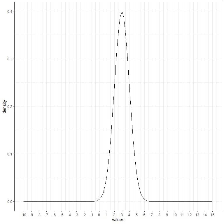
We note that:
- The normal curve is bell-shaped and symmetric around its mean or 3.
- The highest density (peak) is at the mean of 3, and as we move away from 3, the density fades away. It means that data near the mean are more frequent in occurrence than data far from the mean.
- Values greater or less than 3 standard deviation from the mean (values > (3+3X1) =6 or values< (3-3X1)=0) have a density of nearly zero.
We can add another (red) normal curve with mean = 3 and standard deviation = 2.
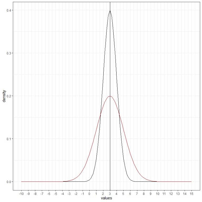
The new red curve is also symmetric and has a peak at 3. In addition, values greater or less than 3 standard deviation from the mean (values > (3+3X2) =9 or values< (3-3X2)= -3) have a density of nearly zero.
The red curve is more flattened than the black curve due to the increased standard deviation.
We can add another (green) normal curve with mean = 3 and standard deviation = 3.
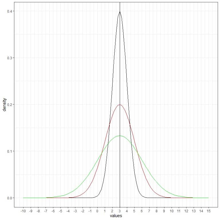
The new green curve is also symmetric and has a peak at 3. Also, values greater or less than 3 standard deviation from the mean (values > (3+3X3) =12 or values< (3-3X3)= -6) have a density of nearly zero.
The green curve is more flattened than the black or red curves due to increased standard deviation.
What will happen if we change the mean and keep the standard deviation constant? Let’s see an example.
– Example 2
The following is a normal distribution for a continuous random variable with mean = 5 and standard deviation = 2.
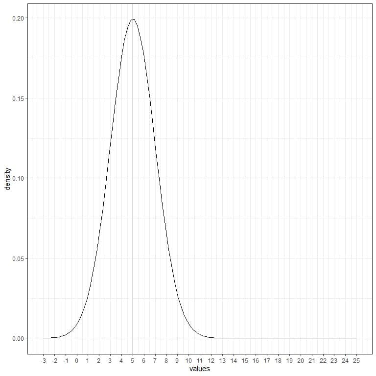
We note that:
- The normal curve is bell-shaped and symmetric around its mean of 5.
- The highest density (peak) is at the mean of 5, and as we move away from 5, the density fades away.
- Values greater or less than 3 standard deviation from the mean (values > (5+3X2) =11 or values< (5-3X2)= -1) have a density of nearly zero.
We can add another (red) normal curve with mean = 10 and standard deviation = 2.
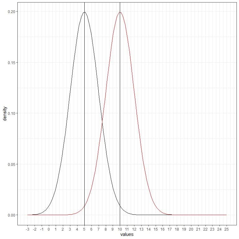
The new red curve is also symmetric and has a peak of 10. Also, values greater or less than 3 standard deviation from the mean (values > (10+3X2) = 16 or values< (10-3X2)= 4) have a density of nearly zero.
The red curve is shifted to the right relative to the black curve.
We can add another (green) normal curve with mean = 15 and standard deviation = 2.
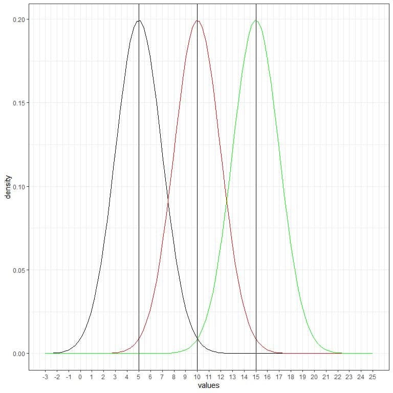
The new green curve is also symmetric and has a peak at 15. Also, values greater or less than 3 standard deviation from the mean (values > (15+3X2) = 21 or values < (15-3X2)= 9) have a density of nearly zero.
The green curve is more shifted to the right relative to the black or red curves.
– Example 3
The age of a certain population has a mean = 47 years and standard deviation = 15 years. Assuming that age from this population follows the normal distribution, we can draw the normal curve for this population’s age.
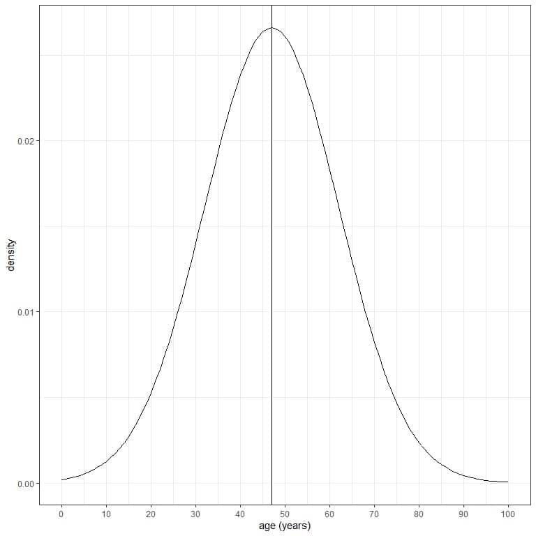
The normal curve is symmetric and has a peak at the mean or 47, and values greater or less than 3 standard deviations from the mean (values > (47+3X15) = 92 years or values < (47-3X15)= 2 years) have a density of nearly zero.
We conclude that:
- Changing the mean of the normal distribution will shift its location to higher or lower values.
- Changing the standard deviation of the normal distribution will increase the spread of the distribution.
The 68-95-99.7% rule
Any normal distribution (curve) follows the 68-95-99.7% rule:
- 68% of the data are within 1 standard deviation from the mean.
- 95% of the data are within 2 standard deviations from the mean.
- 99.7% of the data are within 3 standard deviations from the mean.
It means that for the above population with mean age = 47 years and standard deviation = 15 cm:
1. If we shade the area within 1 standard deviation from the mean or within the mean +/-15 = 47+/-15 = 32 to 62.
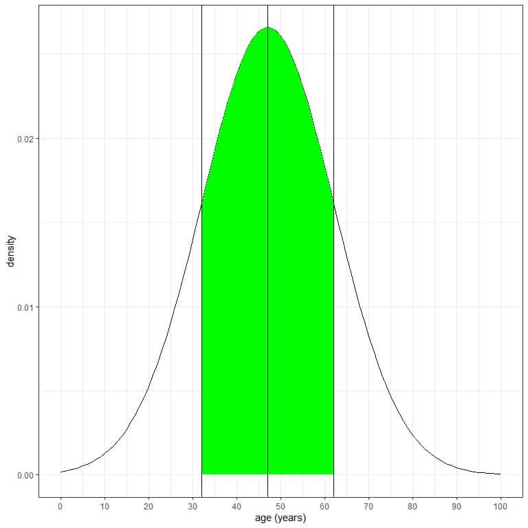
Without integrating for this green AUC, the green shaded area represents 68 % of the total area because it represents data within 1 standard deviation from the mean.
It means that 68% of this population have ages between 32 and 62 years. In other words, the probability of age from this population to lie between 32 and 62 years is 68%.
As the normal distribution is symmetric around its mean, so 34% (68%/2) of this population have age between 47 (mean) and 62 years, and 34% of this population have age between 32 and 47 years.
2. If we shade the area within 2 standard deviations from the mean or within the mean +/-30 = 47+/-30 = 17 to 77.
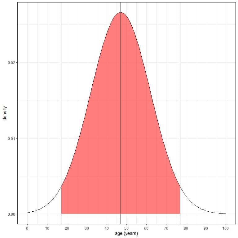
Without doing integration for this red area, the red shaded area represents 95% of the total area because it represents data within 2 standard deviations from the mean.
It means that 95% of this population have ages between 17 and 77 years. In other words, the probability of age from this population to lie between 17 and 77 years is 95%.
As the normal distribution is symmetric around its mean, 47.5% (95%/2) of this population have age between 47 (mean) and 77 years, and 47.5% of this population have age between 17 and 47.
3. If we shade the area within 3 standard deviations from the mean or within the mean +/-45 = 47+/-45 = 2 to 92.
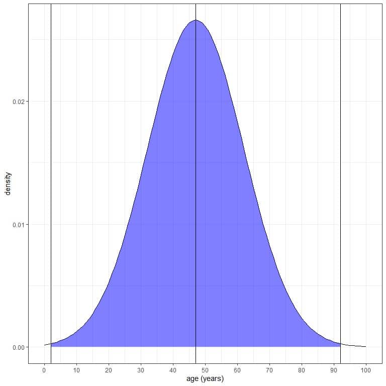
The blue shaded area represents 99.7 % of the total area because it represents data within 3 standard deviations from the mean.
It means that 99.7% of this population have ages between 2 and 92 years. In other words, the probability of age from this population that lies between 2 and 92 years is 99.7%.
As the normal distribution is symmetric around its mean, 49.85% (99.7%/2) of this population have age between 47 (mean) and 92 years, and 49.85% of this population have age between 2 and 47 years.
We can extract other different conclusions from this rule without doing complex integral calculations (to convert the density to probability):
1. The proportion (probability) of data that are larger than the mean = probability of data that are less than the mean = 0.50 or 50%.
In our example of age, the probability that age is less than 47 years = probability that age is greater than 47 years = 50%.
This is plotted as follows:
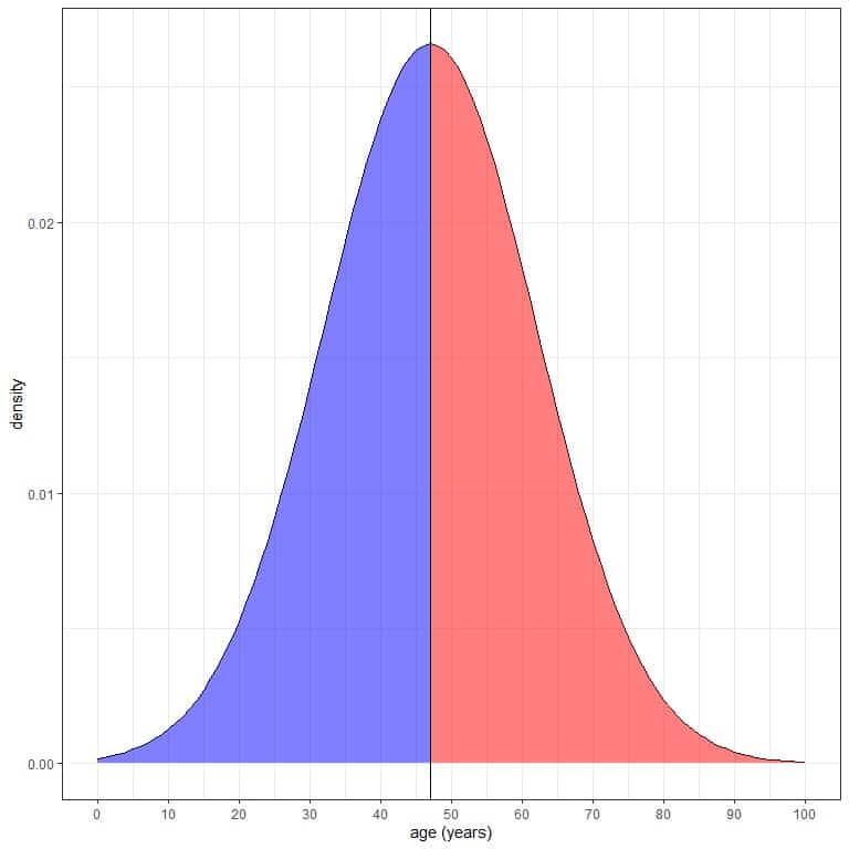
The blue shaded area = probability that age is less than 47 years = 0.5 or 50%.
The red shaded area = probability that age is more than 47 years = 0.5 or 50%.
2. The probability of data that are larger than 1 standard deviation from the mean = (1-0.68)/2 = 0.32/2 = 0.16 or 16%.
In our example of age, the probability that age is greater than (47+15) 62 years = 16%.
3. The probability of data that are smaller than 1 standard deviation from the mean= (1-0.68)/2 = 0.32/2 = 0.16 or 16%.
In our example of age, the probability that age is less than (47-15) 32 years = 16%.
This can be plotted as follows:
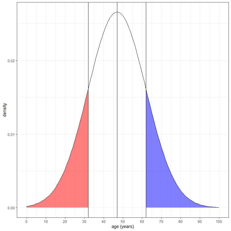
The blue shaded area = probability that age is more than 62 years = 0.16 or 16%.
The red shaded area = probability that age is less than 32 years = 0.16 or 16%.
4. The probability of data that are larger than 2 standard deviation from the mean= (1-0.95)/2 = 0.05/2 = 0.025 or 2.5%.
In our example of age, the probability that age is greater than (47+2X15) 77 years = 2.5%.
5. The probability of data that are smaller than 2 standard deviation from the mean= (1-0.95)/2 = 0.05/2 = 0.025 or 2.5%.
In our example of age, the probability that age is less than (47-2X15) 17 years = 2.5%.
This can be plotted as follows:
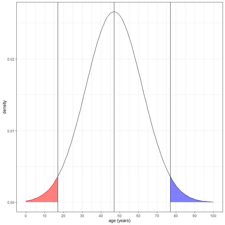
The blue shaded area = probability that age is more than 77 years = 0.025 or 2.5%.
The red shaded area = probability that age is less than 17 years = 0.025 or 2.5%.
6. The probability of data that are larger than 3 standard deviation from the mean= (1-0.997)/2 = 0.003/2 = 0.0015 or 0.15%.
In our example of age, the probability that age is greater than (47+3X15) 92 years = 0.15%.
7. The probability of data that are smaller than 3 standard deviation from the mean= (1-0.997)/2 = 0.003/2 = 0.0015 or 0.15%.
In our example of age, the probability that age is smaller than (47-3X15) 2 years = 0.15%.
This can be plotted as follows:
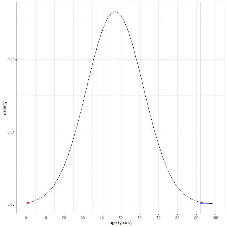
The blue shaded area = probability that age is more than 92 years = 0.0015 or 0.15%.
The red shaded area = probability that age is less than 2 years = 0.0015 or 0.15%.
Both are negligible probabilities.
But do these probabilities correspond to the real probabilities that we observe in our populations or samples?
Let’s see the following example.
– Example 1
The following is the relative frequency table and histogram for heights (in cm) from a certain population.
The mean height of this population = 163 cm and standard deviation = 9 cm.
range | frequency | relative.frequency |
136 – 145 | 40 | 0.02 |
145 – 154 | 390 | 0.17 |
154 – 163 | 785 | 0.35 |
163 – 172 | 684 | 0.30 |
172 – 181 | 305 | 0.14 |
181 – 190 | 53 | 0.02 |
190 – 199 | 2 | 0.00 |
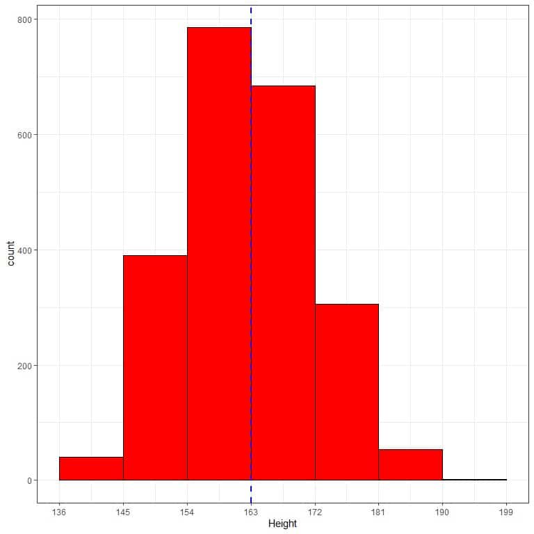
The normal distribution can approximate the histogram of heights from this population because the distribution is nearly symmetric around the mean (163 cm, blue dashed line) and bell-shaped.
In this case, the normal distribution properties (as the 68-95-99.7% rule) can be used to characterize the aspects of this population data.
We will see how the 68-95-99.7% rule give results that are similar to the actual proportion of heights in this population:
1. 68% of the data are within 1 standard deviation from the mean.
The observed proportion for the data within 163 +/-9 = 154 to 172 = relative frequency of 154-163 + relative frequency of 163-172 = 0.35+0.30 = 0.65 or 65%.
2. 95% of the data are within 2 standard deviations from the mean.
The observed proportion for the data within 163 +/-18 = 145 to 181 = sum of relative frequencies within 145-181 =0.17+ 0.35+0.30+0.14 = 0.96 or 96%.
3. 99.7% of the data are within 3 standard deviations from the mean.
The observed proportion for the data within 163 +/-27 = 136 to 190 = sum of relative frequencies within 136-190 =0.02+0.17+ 0.35+0.30+0.14+0.02 = 1 or 100%.
When the histogram of data shows a nearly normal distribution, you can use the normal distribution probabilities to characterize this data’s actual probabilities.
When to use normal distribution?
No real data is perfectly described by the normal distribution because the range of the normal distribution goes from negative infinity to positive infinity, and no real data follows this rule.
However, the distribution of some sample data when plotted as a histogram nearly follows a normal distribution curve (a bell-shaped symmetrical curve centered around the mean).
In this case, the normal distribution properties (as the 68-95-99.7% rule), along with the sample mean and standard deviation, can be used to characterize the aspects of the sample data or the underlying population data if this sample was representative of this population.
– Example 1
The following frequency table and histogram are for the weight in (kg) of 150 participants randomly selected from a certain population.
The mean weight of this sample is 72 kg, and the standard deviation = 14 kg.
range | frequency | relative.frequency |
44 – 58 | 23 | 0.15 |
58 – 72 | 62 | 0.41 |
72 – 86 | 46 | 0.31 |
86 – 100 | 17 | 0.11 |
100 – 114 | 1 | 0.01 |
114 – 128 | 1 | 0.01 |
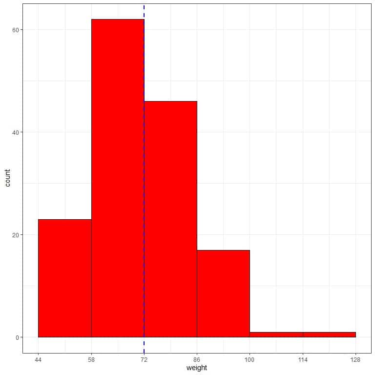
The normal distribution can approximate the histogram of weights from this sample because the distribution is nearly symmetric around the mean (72 kg, blue dashed line) and bell-shaped.
In this case, the properties of the normal distribution can be used to characterize the aspects of the sample or the underlying population:
1. 68% of our sample (or population) have weights within 1 standard deviation from the mean or between (72+/-14) 58 to 86 kg.
The observed proportion in our sample = 0.41+0.31 = 0.72 or 72%.
2. 95% of our sample (population) have weights within 2 standard deviations from the mean or between (72+/-28) 44 to 100 kg.
The observed proportion in our sample = 0.15+0.41+0.31+0.11 = 0.98 or 98%.
3. 99.7% of our sample (population) have weights within 3 standard deviations from the mean or between (72+/-42) 30 to 114 kg.
The observed proportion in our sample = 0.15+0.41+0.31+0.11+0.01 = 0.99 or 99%.
If we apply the normal distribution principles to skewed data, we will get biased or unreal results.
– Example 2
The following frequency table and histogram are for the physical activity in (Kcal/week) of 150 participants randomly selected from a certain population.
This sample’s mean physical activity is 442 Kcal/week, and the standard deviation = 397 Kcal/week.
range | frequency | relative.frequency |
0 – 45 | 10 | 0.07 |
45 – 442 | 83 | 0.55 |
442 – 839 | 34 | 0.23 |
839 – 1236 | 17 | 0.11 |
1236 – 1633 | 3 | 0.02 |
1633 – 2030 | 2 | 0.01 |
2030 – 2427 | 1 | 0.01 |
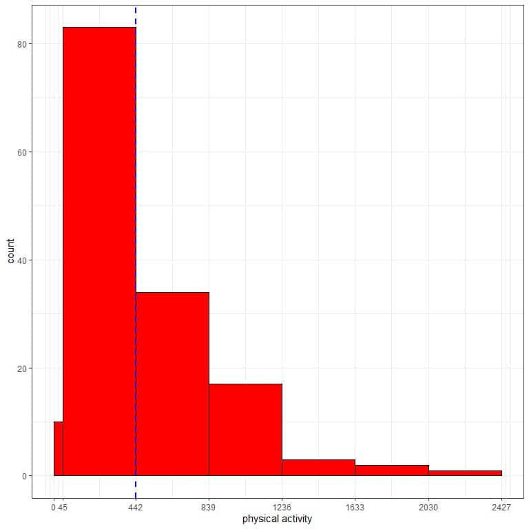
The normal distribution can not approximate the histogram of physical activity from this sample. The distribution is skewed to the right and is not symmetric around the mean (442 Kcal/week, blue dashed line).
Suppose we use the normal distribution properties to characterize the aspects of the sample or the underlying population.
In that case, we will get biased or unreal results:
1. 68% of our sample (or population) have physical activity within 1 standard deviation from the mean or between (442+/-397) 45 to 839 Kcal/week.
The observed proportion in our sample = 0.55+0.23 = 0.78 or 78%.
2. 95% of our sample (population) have physical activity within 2 standard deviations from the mean or between (442+/-(2X397)) -352 to 1236 Kcal/week.
Of course, there is no negative value for physical activity.
It will also be the case for 3 standard deviations from the mean.
Conclusion
For non-normal (skewed data), use the observed proportions (probabilities) of the data as estimates of proportions for the underlying population and do not rely on the normal distribution principles.
We can say that the probability of physical activity to lie between 1633-2030 is 0.01 or 1%.
Normal distribution formula
The normal distribution density formula is:
f(x)=1/(σ√2π) e^((-(x-μ)^2)/(2σ^2 ))
where:
f(x) is the density of the random variable at the value x.
σ is the standard deviation.
π is a mathematical constant. It is approximately equal to 3.14159 and is spelled out as “pi.” It is also referred to as Archimedes’ constant.
e is a mathematical constant approximately equal to 2.71828.
x is the value of the random variable that we want to calculate the density at.
μ is the mean.
How to calculate the Normal distribution?
The formula for the normal distribution density is quite complex to calculate. Instead of calculating the density and integrating the density to obtain probability, R has two main functions for calculating probabilities and percentiles.
For a given normal distribution with mean μ and standard deviation σ:
pnorm(x, mean = μ, sd = σ) gives the probability that values from this normal distribution are ≤ x.
qnorm(p, mean = μ, sd = σ) provides the percentile with below which (pX100)% of the values from this normal distribution falls.
– Example 1
The age of a certain population has a mean = 47 years and standard deviation = 15 years. Assuming that age from this population follows the normal distribution:
1. What is the probability that the age from this population is less than 47 years?
We want the integration of all the area below 47 years which is shaded in blue:
We can use the pnorm function:
pnorm(47, mean = 47, sd=15)
## [1] 0.5
The result is 0.5 or 50%.
We also know that from the normal distribution properties, where the proportion (probability) of data that are larger than the mean = probability of data that are less than the mean = 0.50 or 50%.
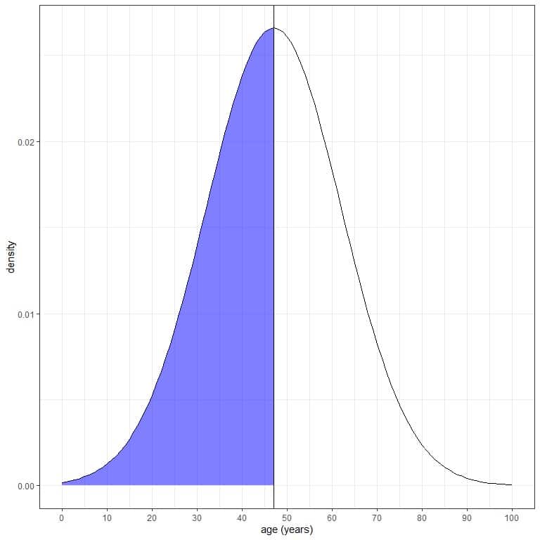
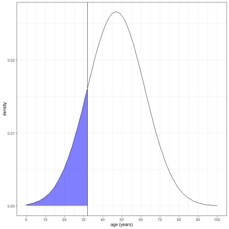
2. What is the probability that the age from this population is less than 32 years?
We want the integration of all the area below 32 years, which is shaded in blue:
We can use the pnorm function:
pnorm(32, mean = 47, sd=15)
## [1] 0.1586553
The result is 0.159 or 16%.
We also know that from the normal distribution properties, since 32 = mean-1Xsd = 47-15, where the probability of data that are larger than 1 standard deviation from the mean = probability of data that are smaller than 1 standard deviation from the mean= 16%.
3. What is the probability that the age from this population is less than 62 years?
We want the integration of all the area below 62 years, which is shaded in blue:
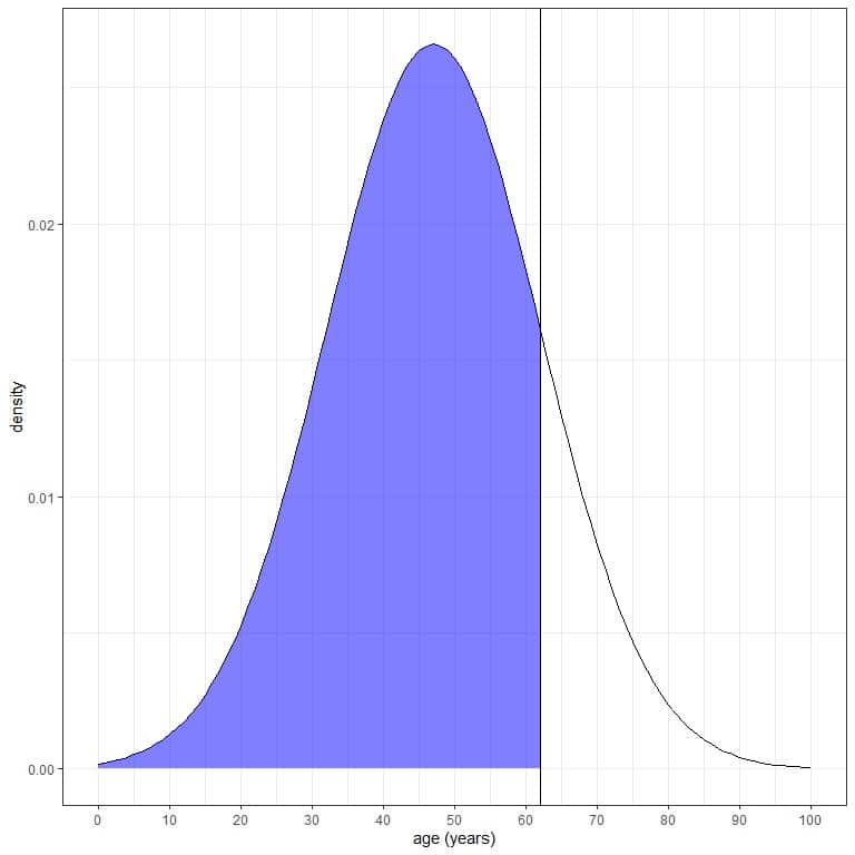
We can use the pnorm function:
pnorm(62, mean = 47, sd=15)
## [1] 0.8413447
The result is 0.84 or 84%.
We also know that from the normal distribution properties, since 62 = mean + 1Xsd = 47+15, where the probability of data that are larger than 1 standard deviation from the mean = probability of data that are smaller than 1 standard deviation from the mean= 16%.
So the probability of data that is larger than 62 = 16%.
Since the total AUC is 1 or 100%, the probability that age is less than 62 is 100-16 = 84%.
4. What is the probability that the age from this population is between 32 and 62 years?
We want the integration of all the area between 32 and 62 years, which is shaded in blue:
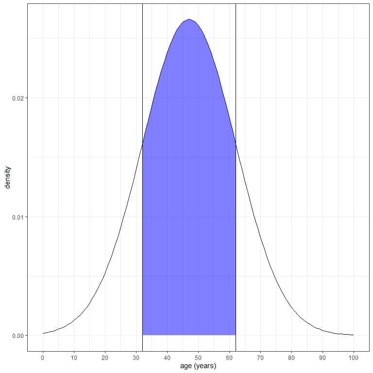
pnorm(62) gives the probability that age is less than 62, and pnorm(32) gives the probability that age is less than 32.
By subtracting pnorm(32) from pnorm(62), we get the probability that age is between 32 and 62 years.
pnorm(62, mean = 47, sd=15)-pnorm(32, mean = 47, sd=15)
## [1] 0.6826895
The result is 0.68 or 68%.
We also know that from the normal distribution properties, where 68% of the data are within 1 standard deviation from the mean.
mean+1Xsd = 47+15=62 and mean-1Xsd = 47-15 = 32.
5. What is the age value below which 25%, 50%, 75%, or 84% of the ages fall?
Using the qnorm function with 25% or 0.25:
qnorm(0.25, mean = 47, sd = 15)
## [1] 36.88265
The result is 36.9 years. So below the age of 36.9 years, 25% of the ages from this population falls below.
Using the qnorm function with 50% or 0.5:
qnorm(0.5, mean = 47, sd = 15)
## [1] 47
The result is 47 years. So below the age of 47 years, 50% of the ages in this population falls below.
We also know that from the properties of the normal distribution because 47 is the mean.
Using the qnorm function with 75% or 0.75:
qnorm(0.75, mean = 47, sd = 15)
## [1] 57.11735
The result is 57.1 years. So below the age 57.1 years, 75% of the ages from this population falls below.
Using the qnorm function with 84% or 0.84:
qnorm(0.84, mean = 47, sd = 15)
## [1] 61.91687
The result is 61.9 or 62 years. So below the age of 62 years, 84% of the ages from this population falls below.
It is the same result as part 3 of this question.
Practice questions
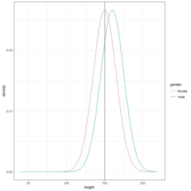
1. The following two normal distributions describe the density of heights (cm) for males and females from a certain population.
Which gender has a higher probability for heights greater than 150 cm (black vertical line)?
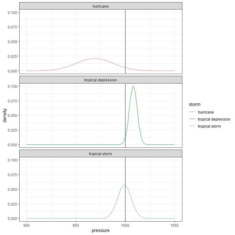
2. The following 3 normal distributions describe the density of pressures (in millibars) for different types of storms.
Which storm has a higher probability for pressures greater than 1000 millibars (black vertical line)?
3. The following table lists the mean and standard deviation for the systolic blood pressure of different smoking habits.
smoker | mean | standard deviation |
Never smoker | 132 | 20 |
Current or former < 1y | 128 | 20 |
Former >= 1y | 133 | 20 |
Assuming that the systolic blood pressure is normally distributed, what is the probability of having less than 120 mmHg (normal level) for each smoking status?
4. The following table lists the mean and standard deviation for the percent poverty in different counties of 3 different USA states (Illinois or IL, Indiana or IN, and Michigan or MI).
state | mean | standard deviation |
IL | 96.5 | 3.7 |
IN | 97.3 | 2.5 |
MI | 97.3 | 2.7 |
Assuming that the percent poverty is normally distributed, what is the probability of having more than 99% percent poverty for every state?
5. The following table lists the mean and standard deviation for hours per day watching TV of 3 different marital statuses in a certain survey.
marital | mean | standard deviation |
Divorced | 3 | 3 |
Widowed | 4 | 3 |
Married | 3 | 2 |
Assuming that the hours per day for watching TV is normally distributed, what is the probability of watching TV between 1 and 3 hours for each marital status?
Answer key
1. Males have a higher probability for heights greater than 150 cm because their density curve has a larger area greater than 150 cm than that for the females’ curve.
2. The tropical depression has a higher probability for pressures greater than 1000 millibars because most of its density curve is larger than 1000 compared to the other storm types.
3. We use the pnorm function along with the mean and standard deviation for every smoking status:
For never smoker:
pnorm(120,mean = 132, sd = 20)
## [1] 0.2742531
The probability = 0.274 or 27.4%.
For the current or former < 1 year: pnorm(120,mean = 128, sd = 20) ## [1] 0.3445783 The probability = 0.345 or 34.5%. For the former >= 1 year:
pnorm(120,mean = 133, sd = 20)
## [1] 0.2578461
The probability = 0.258 or 25.8%.
4. We use the pnorm function along with the mean and standard deviation for every state. Then, subtract the obtained probability from 1 to obtain the probability of larger than 99%:
For state IL or Illinois:
pnorm(99,mean = 96.5, sd = 3.7)
## [1] 0.7503767
The probability = 0.75 or 75%. The probability of more than 99% percent poverty in Illinois is 1-0.75 = 0.25 or 25%.
For state IN or Indiana:
pnorm(99,mean = 97.3, sd = 2.5)
## [1] 0.7517478
The probability = 0.752 or 75.2%. So, the probability of more than 99% percent poverty in Indiana is 1-0.752 = 0.248 or 24.8%.
For state MI or Michigan:
pnorm(99,mean = 97.3, sd = 2.7)
## [1] 0.7355315
so the probability = 0.736 or 73.6%. So the probability of more than 99% percent poverty in Indiana is 1-0.736 = 0.264 or 26.4%.
5. We use the pnorm(3) function along with the mean and standard deviation for every state. Then, subtract the pnorm(1) from it to obtain the probability of watching TV between 1 and 3 hours:
For divorced status:
pnorm(3,mean = 3, sd = 3)- pnorm(1,mean = 3, sd = 3)
## [1] 0.2475075
The probability = 0.248 or 24.8%.
For widowed status:
pnorm(3,mean = 4, sd = 3)- pnorm(1,mean = 4, sd = 3)
## [1] 0.2107861
The probability = 0.211 or 21.1%.
For married status:
pnorm(3,mean = 3, sd = 2)- pnorm(1,mean = 3, sd = 2)
## [1] 0.3413447
The probability = 0.341 or 34.1%. The married status has the highest probability.