Riemann Sum – Two Rules, Approximations, and Examples
 The Riemann sum is the first approximation method that we’ll be learning in our Integral calculus classes. This approximation method allows us to estimate the area under a curve or a graph.
The Riemann sum allows us to approximate the area under the curve by breaking the region into a finite number of rectangles. We can also use the Riemann sum as a way to define the integration operation.
Through the fundamental theorem of calculus, we’ve learned that the definite integral of a function over $[a, b]$ represents the area of the function’s curve. There are instances, however, that we need to approximate the integral instead. The Riemann sum shows us one way of estimating the area under the curve is by combining the area of a finite number of rectangles.
In this article, we’ll show you how to approximate the definite integral through the Riemann sum. We’ll also show you two types of approximation: the right-hand rule and the left-hand rule.
What is a Riemann sum?
The Riemann sum utilizes a finite number of rectangles to approximate the value of a given definite integral. We can define the Riemann sum as the sum of these $ n$ rectangles’ areas.
Let’s take a look at non-negative function, $f(x)$, that is continuous within the closed interval, $[a, b]$.
Through the Riemann sum, it’s now possible for us to approximate the area of the region found right below the curve. This area is bounded by the $x$-axis as well as the vertical lines: $x =a$ and $x = b$.
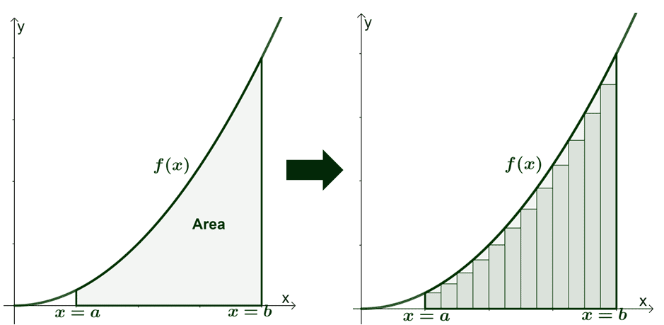
Here’s an example of how a definite integral, $\int_{a}^{b} f(x)\phantom{x}dx$, can be approximated by breaking down the area under the curve of $f(x)$ as a sum of the rectangles’ areas.
Riemann sum definition
We can divide the region under the curve and bounded by the interval, $[a, b]$. When we use $n$ rectangles to divide the region, each subinterval is expected to have a width of $\Delta x$.
The areas of the $\boldsymbol{n}$ rectangles can then be added to estimate the area of the entire region.
\begin{aligned}\text{Area of rectangle} &= \sum_{i =0}^{n – 1} f(x_i) \Delta x\end{aligned}
In the second part of the fundamental theorem of calculus, we’ve learned that the definite integral, $\int_{a}^{b}f(x)\phantom{x} dx$, represents the area under $f(x)$’s curve and bounded by $x = a$ and $x = b$.
This confirms the definition of Riemann sum: an approximation of the definite integral, $\int_{a}^{b}f(x)\phantom{x} dx$, by adding the rectangles that divide the region into $n$ subintervals.
\begin{aligned} \int_{a}^{b}f(x)\phantom{x} dx &\approx \lim_{n \rightarrow \infty}\sum_{i =0}^{n – 1} f(x_i) \Delta x\\&\approx f(x_1)\Delta x + f(x_2)\Delta x + f(x_3)\Delta x + …+ f(x_n)\Delta x\end{aligned}
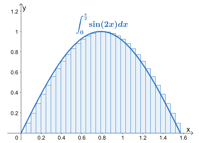
The graph shown above is a good example of how we can break down the region for $\int_{0}^{\frac{\pi}{2}} \sin 2x \phantom{x} dx$ into $30$ rectangles with uniform widths.
The index in the summation notation shown may change depending on whether we’re working with a left-hand or right-hand Riemann sum. We’ll learn more about these two in the next section.
How to do Riemann sum?
Before we discuss the process of constructing and evaluating the Riemann, let us show you the difference between the right-hand rule and the left-hand rule for the Riemann sum.
- In the right Riemann sum, we construct the rectangles so that the curve passes through the top-right right corners.
Similarly, for the left Riemann sum, we construct the rectangles so that the curve passes through the top-left corners.
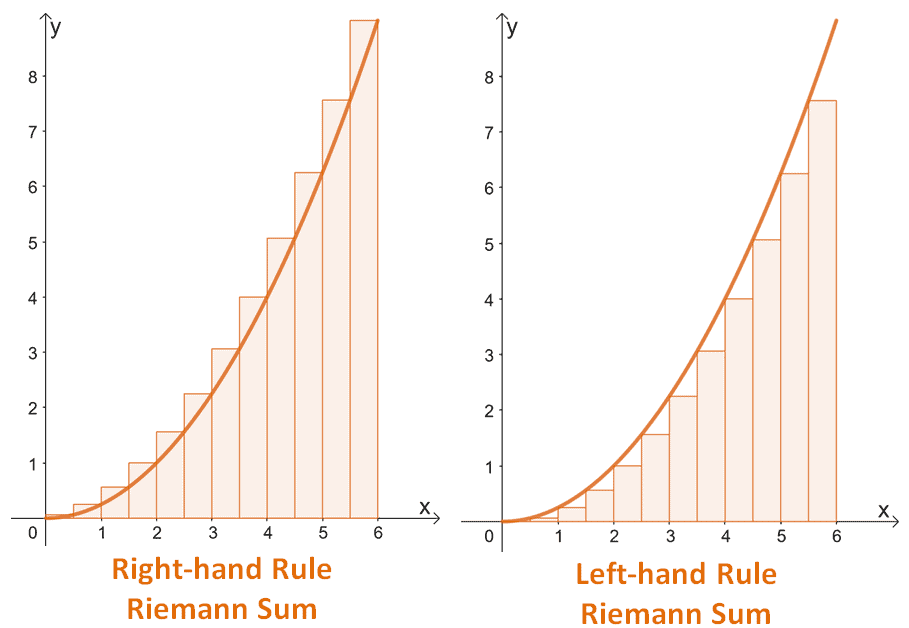
These two graphs highlight this difference between the right and left Riemann sums. The curve passes through each of the top-right corners for the right Riemann sum while it passes through the top-left corners for the left-hand Riemann sum.
Because of this difference, the process of writing $\int_{a}^{b} f(x) \phantom{x} dx$’s right and left Riemann sums in summation notation will differ slightly too. Let us summarize the steps for you here:
Step 1: Establish the value of $\Delta x$. Recall that $\Delta x$ represents the width of the rectangle. Using the definite integral’s lower and upper limits, we have $\Delta x = \dfrac{b -a}{n}$.
Step 2: Find the endpoints of the rectangles. Let $x_i$ represent each of the endpoints.
Step 3: Express the area of the rectangle in terms of $\Delta x$ and $f(x_i)$. Each rectangle will have an area of $\Delta x \cdot f(x_i)$.
Step 4: Using the definition of the Riemann sum, we then add all the areas from Step 3. This is when the summation notation comes in handy. This step will also show you how the right and left Riemann sums would differ.
- The endpoints of the right-hand rule for the Riemann sum will have endpoints at $\{x_1, x_2, x_3,…, x_{n -1}, x_n\}$.
- Meanwhile, the left-hand rule will have endpoints at $\{x_0, x_1, x_2, …, x_{n -2}, x_{n -1}\}$.
- Keep in mind that $x_0 = a$ and $x = b$, where $a$ and $b$ are the definite integral’s upper and lower limits.
This makes sense because as we have mentioned in the earlier section, the integral’s curve will pass through the right and left Riemann sum’s rectangles at their top right and left corners, respectively.
Hence, we have the following right and left Riemann sum’s summation notation:
| Right Riemann Sum | Left Riemann Sum |
| \begin{aligned}\sum_{i = 1}^{n} \Delta x \cdot f(x_i) \end{aligned} | \begin{aligned}\sum_{i = 0}^{n – 1} \Delta x \cdot f(x_i) \end{aligned} |
The two formulas confirm that the summation notations of the right and left Riemann sums only differ by the index: the right-hand rule begins with $i = 1$ while the left-hand rule begins with $i = 0$.
To approximate the total area under the definite interval’s curve using the Riemann sum, evaluate $\{f(x_i)\}$ each time then add the total values. Multiply this sum to the width, $\Delta x$.
| Right Riemann Sum | Left Riemann Sum |
| \begin{aligned}\Delta x[f(x_1) + f(x_2) + …f(x_n)] \end{aligned} | \begin{aligned}\Delta x[f(x_0) + f(x_1) + …f(x_{n – 1})] \end{aligned} |
To evaluate the Riemann sum, expand the summation notation. There are instances when you might need to apply some properties of the summation notation or sigma notation:
| Helpful Summation Properties |
| \begin{aligned}\sum_{i = 1}^{n} k &= k\\\sum_{i = 1}^{n} ka_i &= k\sum_{i = 1}^{n} a_i\\\sum_{i = 1}^{n} (a_i + b_i) &= \sum_{i = 1}^{n} a_i + \sum_{i = 1}^{n} b_i\\\sum_{i = 1}^{n} (a_i – b_i) &= \sum_{i = 1}^{n} a_i – \sum_{i = 1}^{n} b_i\end{aligned} |
Use these properties to simplify the process of evaluating complex summation notations. When asked to graph the definite integral’s Riemann sum, we follow the following steps:
- Create rectangles with each rectangle having a width of $\Delta x$.
- Evaluate $x_i$ at $f(x)$ to determine the height of each of the rectangle.
- Use the definition of the left-hand and right-hand Riemann sum to know the corners that the function’s passes through.
Example of writing a Riemann sum formula
Let’s go ahead and show you how the definite integral, $\int_{0}^{2} 4 – x^2 \phantom{x}dx$, can be written in left and right Riemann sum notations with four rectangles.
We first determine the value of $\Delta x$ by dividing $2- 0$ by $4$.
\begin{aligned}\Delta x &= \dfrac{2 – 0}{4}\\&= \dfrac{1}{2}\end{aligned}
We then take note of the right and left Riemann sums’ endpoints. Keep in mind that $x_0 = 0$ and $x_4 = 2$.
- For the left-hand rule, we begin with $x_0 = 0$ then add $\dfrac{1}{2}$ to find the next endpoint. Hence, we have $x_i = \left\{0, \dfrac{1}{2}, 1, dfrac{3}{2}\right\}$.
- For the right-hand rule, we start with $x_1 = \dfrac{1}{2}$ then increase it by $\dfrac{1}{2}$ for each successive endpoint. This means that we have $x_i = \left\{\dfrac{1}{2}, 1, dfrac{3}{2}, 2\right\}$.
Apply the formula for the Riemann sum using the right-hand and left-hand rules to approximate the area under the curve of $\int_{0}^{2} 4 – x^2 \phantom{x}dx$.
| Right Riemann Sum | Left Riemann Sum |
| \begin{aligned}\sum_{i = 1}^{4} \Delta x \cdot f(x_i) &= \dfrac{1}{2}\left[f\left(\dfrac{1}{2}\right ) + f(1) + f\left(\dfrac{3}{2}\right) + f(2)\right ]\\&= \dfrac{1}{2}\left(\dfrac{15}{4}+ 3 + \dfrac{7}{4}+0 \right )\\&=4.25 \end{aligned} | \begin{aligned}\sum_{i = 0}^{3} \Delta x \cdot f(x_i) &= \dfrac{1}{2}\left[f(0) + f\left(\dfrac{1}{2}\right ) + f(1) + f\left(\dfrac{3}{2}\right)\right ]\\&= \dfrac{1}{2}\left(4+ \dfrac{15}{4}+ 3 + \dfrac{7}{4}\right )\\&=6.25 \end{aligned} |
The actual value of $\int_{0}^{2} 4 – x^2 \phantom{x} dx$ is $\dfrac{15}{3}$ and our approximated values through the right-hand rule and the left-hand rule are $4.25$ and $6.25$, respectively.
Another form of the Riemann sum is the midpoint rule, but we’ll learn about this when we discuss other methods of approximating integrals.
Example of sketching a Riemann sum graph
What if we’re asked to sketch the definite integral with the region below divided by the Riemann sum’s rectangles? We can use the values of $\Delta x$ and $f(x_i)$ to represent the Riemann sum.
- Divide the interval, $[a, b]$, into $n$ rectangles with a width of $\Delta x$.
- Determine the height of each of the rectangle by evaluating $f(x_i)$.
- Double-check if the curve of $f(x)$ passes through the right corners of the rectangles.
Let’s use $\int_{0}^{2} 4 – x^2 \phantom{x}dx$, for example. We want $4$ rectangles with a width of $\dfrac{1}{2}$ unit. Here’s how the graphs of the left and right Riemann sum for this particular definite integral.
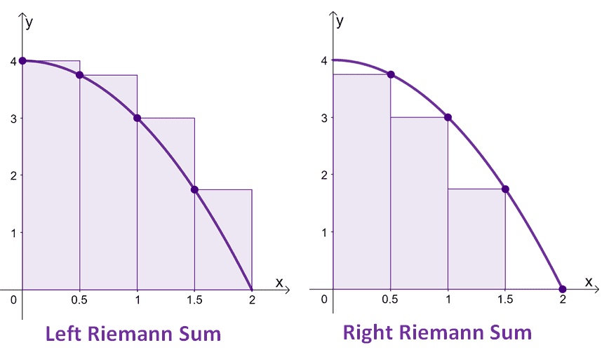
This shows that left Riemann sum passes through the top-left corners at $x = \{0, 0.5, 1, 1.5\}$. The right Riemann sum passes through the top-right corners at $x = \{0.5, 1, 1.5, 2\}$. Notice how the right Riemann sum appears to only have three rectangles instead of four? That’s because at the last endpoint (or when $x = 2$), $f(2)$ is equal to $0$.
Example 1
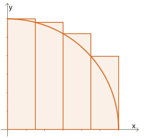
Approximate the Riemann sum shown below. Keep in mind that the graph shows a left-hand approximation of the area under the function shown below.
\begin{aligned}f(x) &= \sqrt{9 – x^2}\phantom{x}dx,\phantom{xx} 0 \leq x \leq 3\end{aligned}.
Solution
The graph above shows us that the area under the region will be divided into four subintervals. This means that each rectangle will have a width shown below.
\begin{aligned}\Delta x &= \dfrac{3 – 0}{4}\\&= \dfrac{3}{4}\end{aligned}
Since we’re performing a left Riemann sum approximation, we’re going to evaluate $f(x)$ at the following values:
\begin{aligned}x_0 &= 0\\x_1 &= \dfrac{3}{4}\\x_2 &= \dfrac{3}{2}\\x_3 &= \dfrac{9}{4}\end{aligned}
Approximate the function’s left Rieman sum using the formula, $\sum_{i =0}^{n -1} f(x_i)\Delta x$, where $n = 4$.
\begin{aligned}f(0) &= \sqrt{9 -0^2}\\&= 3\\f\left(\dfrac{3}{4} \right )&= \sqrt{9 – \dfrac{3}{4}^2}\\&\approx 2.9047\\f\left(\dfrac{3}{2} \right )&= \sqrt{9 – \dfrac{3}{2}^2}\\&\approx 2.5981\\f\left(\dfrac{9}{4} \right )&= \sqrt{9 – \dfrac{9}{4}^2}\\&\approx 1.9843\end{aligned}
Approximate the left Riemann sum by adding these values and multiplying the sum by $\Delta x = \dfrac{3}{4}$.
\begin{aligned}\int_{0}^{3} \sqrt{9 – x^2}\phantom{x}dx &\approx \Delta x[f(x_0) + f(x_1) + f(x_2)+ f(x_3)] \\& = \dfrac{3}{4}\left[f(0)+ f\left(\dfrac{3}{4}\right) + f\left(\dfrac{3}{2}\right) +f\left(\dfrac{9}{4}\right) \right ]\\&= \dfrac{3}{4}(3 + 2.9047+ 2.5981 + 1.9843)\\&\approx 7.8653\end{aligned}
Using the graph and the left-hand rule for the Riemann sum, we have approximated $\int_{0}^{3} \sqrt{9 -x^2}\phantom{x}dx$ as $7.8653$.
Example 2
Evaluate the Riemann sum for the function, $g(x)= x^4 – 4x$, using the top right corners of the curve that is bound by the following limits: $x=0$ and $x = 2$. Divide the region by $n = 8$ rectangles.
Solution
Since we want the curve of $g(x)$ to pass through the top right corners of the rectangles, we’re evaluating a right Riemann sum. Now, identify the width of the rectangle and the key endpoints that we need to focus on:
- Calculate the width of each of the $8$ rectangles and express it as $\Delta x$.
\begin{aligned}\Delta x &= \dfrac{2 – 0}{8}\\&= 0.25\end{aligned}
- Take note of the endpoints with $x_0$ as the first endpoint and $x_8$ as the last endpoint.
\begin{aligned}x_0 &=0 \\x_1 &=0.25\\x_2 &= 0.50\\x_3&=0.75\\x_4&= 1.00\\x_5 &= 1.25\\x_6 &= 1.50\\x_7&= 1.75\\x_8 &= 2.00\end{aligned}
- Since we’re working with the right-hand rule for the Riemann sum, we’ll evaluate $g(x)$ from $x_1$ to $x_8$.
When approximating a right Riemann sum, we use the formula, $\begin{aligned}\sum_{i = 1}^{n} \Delta x \cdot f(x_i) \end{aligned}$. Hence, we have the following expression for the right Riemann sum approximation:
\begin{aligned}\int_{0}^{2} x^4 – 4x\phantom{x}dx &= \sum_{i =1}^{8} \Delta x \cdot g(x_i)\\&= \dfrac{1}{4}[g(0.25)+g(0.50)+ g(0.75) +g(1.00) +\\&\phantom{xxxx} g(1.25) +g(1.50) + g(1.75)+ g(2.00)]\\&\approx \dfrac{1}{4}(-0.9961 -1.9375 -2.6836 -3- 2.5586- 0.9375 +2.3789+ 8)\\&\approx -0.4336\end{aligned}
Hence, we have the right Riemann sum approximated to be $-0.4336$.
Example 3
Use the results from Example 2 to graph the curve of $g(x)$ and the rectangles representing the right Riemann sum approximation. From the graph, explain why the definite integral is negative.
Solution
Use the evaluated values of $g(x)$ from the given endpoints in Example 2. This will guide us in graphing $g(x)$’s curve.
| \begin{aligned}\boldsymbol{x_i}\end{aligned} | \begin{aligned}\boldsymbol{g(x_i)}\end{aligned} |
| \begin{aligned}x_1 &= 0.25\end{aligned} | \begin{aligned}g(x_1) &= -0.9961\end{aligned} |
| \begin{aligned}x_2 &= 0.50\end{aligned} | \begin{aligned}g(x_2) &= -1.9375\end{aligned} |
| \begin{aligned}x_3 &= 0.75\end{aligned} | \begin{aligned}g(x_3) &= -2.6836\end{aligned} |
| \begin{aligned}x_4 &= 1.00\end{aligned} | \begin{aligned}g(x_4) &= -3\end{aligned} |
| \begin{aligned}x_5 &= 1.25\end{aligned} | \begin{aligned}g(x_5) &= -2.5586\end{aligned} |
| \begin{aligned}x_6 &= 1.50\end{aligned} | \begin{aligned}g(x_6) &= -0.9375\end{aligned} |
| \begin{aligned}x_7 &= 1.75\end{aligned} | \begin{aligned}g(x_7) &= 2.3789\end{aligned} |
| \begin{aligned}x_8 &= 2.00\end{aligned} | \begin{aligned}g(x_8) &= 8\end{aligned} |
These are also the points on the rectangle that the curve will be passing through.
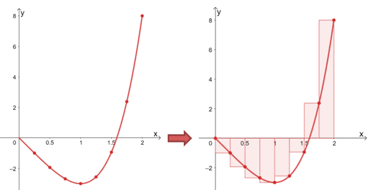
Construct eight rectangles with a uniform with of $\Delta x = 0.25$ unit. The height of each rectangle will depend on the values returned by $g(x)$. To confirm that the rectangles you’ve constructed are correct, see if the curve passes through each of the rectangle’s top right corners.
Recall that the right Riemann sum is approximated to be $-0.4336$ and the graph highlights how a Riemann sum can be negative. Since the rectangles are found below the $x$-axis, the definite integral at this interval, $[0, 1.5]$, is negative. To find the total area, we simply subtract the area found below the $\boldsymbol{x}$-axis from the area found above the $\boldsymbol{x}$-axis.
Example 4
Estimate the area between the function, $f(x) = x^2 – 4x + 4$ and the $x$-axis within the interval, $[0, 4]$. Use $n = 6$ rectangles to estimate the area and the two Riemann sum rules:
a. Approximate using the left Riemann sum.
b. Approximate using the right Riemann sum.
Solution
The two Riemann sum rules will utilize the same width for their rectangles: $\Delta x = \dfrac{4 – 0}{5} = 0.8$ unit. Let’s go ahead and begin with $x_0 = 0$ and add $0.8$ to find the next endpoint until we reach $x_5 = 4$.
\begin{aligned}x_0 &= 0\\x_1 &= 0.8\\x_2 &= 1.6\\x_3 &= 2.4\\x_4 &= 3.2\\x_5 &= 4\end{aligned}
We’ll use the products of $\Delta x = 0.8$ and $f(x_i)$ then add the results together. Here’s the table of values for $f(x_i)$ from $x_0 = 0$ to $x_5 = 4$:
| \begin{aligned}\boldsymbol{x_i}\end{aligned} | \begin{aligned}\boldsymbol{f(x_i)}\end{aligned} | \begin{aligned}\boldsymbol{x_i}\end{aligned} | \begin{aligned}\boldsymbol{f(x_i)}\end{aligned} |
| \begin{aligned}x_0 &= 0\end{aligned} | \begin{aligned}f(0) &= 4\end{aligned} | \begin{aligned}x_3 &= 2.4\end{aligned} | \begin{aligned}f(2.4) &= 0.16\end{aligned} |
| \begin{aligned}x_1 &= 0.8\end{aligned} | \begin{aligned}f(0.8) &= 1.44\end{aligned} | \begin{aligned}x_4 &= 3.2\end{aligned} | \begin{aligned}f(3.2) &= 1.44\end{aligned} |
| \begin{aligned}x_2 &= 1.6\end{aligned} | \begin{aligned}f(1.6) &= 0.16\end{aligned} | \begin{aligned}x_5 &= 4\end{aligned} | \begin{aligned}f(4) &= 4\end{aligned} |
The difference between the two rules is the positions that the curve passes through and the range of values for $\boldsymbol{i}$ in their summation notation.
Let’s work on the left-hand rule first:
- The graph of $f(x)$ will pass through the top-left corners of the rectangles.
- The summation notation for the left Riemann sum is $\sum_{i=0}^{i = n -1} \Delta x(x_i)$.
- This means that we’ll use $\Delta x = 0.8$ and $\{f(x_0), f(x_1), f(x_2), f(x_3), f(x_4)\}$.
The area bounded by $f(x)$ and the $x$-axis can be estimated by the left Riemann sum as shown below:
\begin{aligned}\text{Area}&=\sum_{i =0}^{4} \Delta x \cdot f(x_i)\\&= 0.8[f(0) + f(0.8) + f(1.6) + f(2.4) + f(3.2)]\\&\approx 0.8(4 + 1.44 + 0.16 + 0.16 +1.44)\\&\approx 5.76\end{aligned}
a. This means that the area under curve, through the left Riemann sum, is approximately equal to $5.76$ squared units.
We’ll apply a similar process for the right-hand rule but this time, we’ll use $\Delta x = 0.8$ and $\{f(x_1), f(x_2), f(x_3), f(x_4), f(x_5)\}$. We can approximate the area as shown below.
\begin{aligned}\text{Area}&=\sum_{i =1}^{5} \Delta x \cdot f(x_i)\\&= 0.8[f(0.8) + f(1.6) + f(2.4) + f(3.2) + f(4)]\\&\approx 0.8(1.44 + 0.16 + 0.16 +1.44+ 4)\\&\approx 5.76\end{aligned}
b. Through the right Riemann sum, the area is approximately equal to $5.76$ squared units.
Example 5
Compare the relative error of approximating the definite integral, $\int_{0}^{4} x^2 – 4x + 4\phantom{x}dx$, using the left and right Riemann sums and the fact that the actual value of the definite integral is equal to $\dfrac{16}{3}$.
Hint: The relative error can be calculated using the formula shown below. \begin{aligned}\text{Relative Error}&= \dfrac{|\text{Actual Value} – \text{Approximated Value}|}{\text{Actual Value}} \times 100\%\end{aligned}
Solution
We can approximate the definite integral, $\int_{0}^{4} x^2 -4x + 4\phantom{x}dx$, using the Riemann sums from Example 4. Both the right and left-hand rules returned an approximation of $5.76$ squared units.
| Approximating Definite Integral Using Left Riemann Sum | Approximating Definite Integral Using Right Riemann Sum |
\begin{aligned}\int_{a}^{b} f(x) \phantom{x} dx & \approx \sum_{i =0}^{n -1}\Delta x \cdot f(x_i)\end{aligned}
| \begin{aligned}\int_{a}^{b} f(x) \phantom{x} dx & \approx \sum_{i = i}^{n}\Delta x \cdot f(x_i)\end{aligned}
|
This means that for both left and right Riemann sum approximations, we have $\int_{0}^{4} x^2 – 4x + 4 \phantom{x} dx \approx 5.76$. Let’s now calculate the relative error since we have both the actual and approximated values.
\begin{aligned}\text{Relative Error}&= \dfrac{\left|\dfrac{16}{3} – 5.76\right|}{\dfrac{16}{3}} \times 100\%\\&\approx 8.00\%\end{aligned}
Hence, the relative error for both approximations is $8.00\%$.
Practice Questions
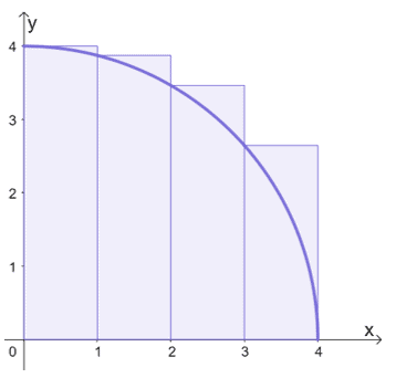
1. Approximate the Riemann sum shown below. Keep in mind that the graph shows a left-hand approximation of the area under the function shown below.
\begin{aligned}f(x) &= \sqrt{16 – x^2}\phantom{x}dx,\phantom{xx} 0 \leq x \leq 4\end{aligned}.
2. Evaluate the Riemann sum for the function, $g(x)= x^5 – 6x$, using the top right corners of the curve that is bound by the following limits: $x=0$ and $x = 3$. Divide the region by $n = 6$ rectangles. Approximate the value to four decimal places.
3.Estimate the area between the function, $f(x) = x^2 – 6x + 9$ and the $x$-axis within the interval, $[0, 3]$. Use $n = 6$ rectangles to estimate the area and the two Riemann sum rules:
a. Approximate using the left Riemann sum.
b. Approximate using the right Riemann sum.
4.Calculate the relative errors for Question 3 given that the actual value of $\int_{0}^{3} x^2 – 6x + 9\phantom{x} dx$ is equal to $9$ squared units. Using the results, which would be a better approximation for the definite integral?
5. Estimate the area between the function, $g(x) = x^3 – 2x + x + 1$ and the $x$-axis within the interval, $[0, 5]$. Use $n = 8$ rectangles to estimate the area and the two Riemann sum rules:
a. Approximate using the left Riemann sum (three decimal places).
b. Approximate using the right Riemann sum (three decimal places).
6.Calculate the relative errors for Question 5 given that the actual value of $\int_{0}^{5} x^3 – 2x + x + 1\phantom{x} dx$ is equal to $148.75$ squared units. Using the results, which would be a better approximation for the definite integral?
7. Evaluate the Riemann sum for $f(x) = 3x^2$ throughout the interval, $[0, 5]$ that uses the left endpoint and the following:
a. $10$ identical subintervals
b. $100$ identical subintervals.
Approximate the values to three decimal places.
8. Evaluate the Riemann sum for $g(x) = 4x^2$ throughout the interval, $[0, 8]$ that uses the right endpoint and the following:
a. $10$ identical subintervals
b. $100$ identical subintervals.
Approximate the values to two decimal places.
Answer Key
1. $\int_{0}^{4}\sqrt{16 – x^2}\phantom{x}dx \approx 12.73571$
2. $\int_{0}^{3} x^5 – 6x \phantom{x}dx \approx 159.1406$
3.
a. $\sum_{i = 0}^{5} \Delta x f(x_i) = 11.375$
b. $\sum_{i = 1}^{6} \Delta x f(x_i) = 6.875$
4.
| Relative Errors | |
| Left Riemann Sum | \begin{aligned} 26.39\%\end{aligned} |
| Right Riemann Sum | \begin{aligned} 23.61\%\end{aligned} |
Since the relative error is smaller for the right Riemann sum, it was a better approximation.
5.
a. $\sum_{i = 0}^{5} \Delta x g(x_i) = 113.691$
b. $\sum_{i = 1}^{8} \Delta x g(x_i) = 188.691$
6.
| Relative Errors | |
| Left Riemann Sum | \begin{aligned} 23.57\%\end{aligned} |
| Right Riemann Sum | \begin{aligned} 26.85\%\end{aligned} |
Since the relative error is smaller for the left Riemann sum, it was a better approximation.
7.
a. $ \int _0^5\:3x^2\:dx \approx 106.875$
b. $ \int _0^5\:3x^2\:dx \approx 123.131$
8.
a. $ \int _0^8\:4x^2\:dx \approx 583.68 $
b. $ \int _0^8\:4x^2\:dx \approx 672.46$
Images/mathematical drawings are created with GeoGebra.