The Sample Mean – Explanation & Examples

The definition of the sample mean is:

“The sample mean is the mean or average found in a sample.”

In this topic, we will discuss the sample mean from the following aspects:

• What is the sample mean?
• How to find the sample mean?
• The sample mean formula.
• Properties of the sample mean.
• Practice questions.
• Answer key.

What is the sample mean?

The sample mean is the mean value of a numerical characteristic of a sample. The sample is a subset of a larger group or population. We collect information from a sample to learn about the larger group or population.

The population is the entire group we want to study. However, collecting information from the population may not be possible in many cases due to the great resources it needs.

For example, if we want to study the heights of American males. We can survey every American male and get his height. This is population data.

Alternatively, we can select 200 American males and measure their heights. This is sample data.

If we calculate the mean of the population data, its symbol is the Greek letter μ and pronounced “mu.”

If we calculate the mean of the sample data, its symbol is ¯x and pronounced “x bar.”
We use the sample mean ¯x as an estimate of the population mean μ to save a lot of money and time.

When the sample is representative of the population under study, the sample mean will be a good estimator of the population mean.

When the sample is not representative of the population, the sample mean will be a biased estimator of the population mean.

One example of a representative sampling strategy is simple random sampling. Each member of the population is assigned a number. Then using a computer program, you can select a random subset of any size.

How to find the sample mean?

We will go through several examples.

– Example 1

Suppose we want to study the age of a certain population. Because of limited resources, only 20 individuals are randomly selected from the population, and we have their ages in years. What is the mean of this sample?

1. Add up all of the numbers:

70 + 56 + 37 + 69 + 70 + 40 + 66 + 53 + 43 + 70 + 54 + 42 + 54 + 48 + 68 + 48 + 42 + 35 + 72 + 70 = 1107.

2. Count the numbers of items in your sample. In this sample, there are 20 items or 20 participants.

3. Divide the number you found in Step 1 by the number you found in Step 2.

The sample mean = 1107/20 = 55.35 years.

Note that the sample mean has the same unit as the original data.

– Example 2

Suppose we want to study the weights of a certain population. Because of limited resources, only 25 individuals are surveyed, and we have their weights in kg. What is the mean of this sample?

1. Add up all of the numbers:

64.0 +67.0 +70.0 +68.0+ 43.5 +79.2 +45.8 +53.0 +62.0 +79.0 +66.0 +65.0 +60.0 +69.0+ 69.0+ 88.0+ 76.0+ 69.0+ 80.0+ 77.0+ 63.4+ 72.0+ 65.5+ 75.0+ 84.0 = 1710.4.

2. Count the numbers of items in your sample. In this sample, there are 25 items.

3. Divide the number you found in Step 1 by the number you found in Step 2.

The sample mean = 1710.4/25 = 68.416 kg.

– Example 3

Suppose we want to study the heights of a certain population. Because of limited resources, only 36 individuals are surveyed, and we have their heights in cm. What is the mean of this sample?

1. Add up all of the numbers:

160.0+ 163.0+ 170.0+ 147.0+ 158.0+ 164.0+ 154.5+ 160.0+ 160.0+ 163.0+ 160.0+ 167.0+ 150.0+ 156.0+ 157.0+ 180.0+ 163.0+ 155.0+ 156.0+ 162.0+ 155.5+ 155.0+ 158.5+ 172.0+ 174.0+ 161.0+ 153.0+ 169.0+ 167.0+ 170.0+ 159.0+ 164.5+ 169.0+ 160.0+ 158.0+ 162.0 = 5813.

2. Count the numbers of items in your sample. In this sample, there are 36 items.

3. Divide the number you found in Step 1 by the number you found in Step 2.

The sample mean = 5813/36 = 161.4722 cm.

– Example 4

Suppose we want to study the weights of a certain collection of more than 50,000 diamonds. Instead of weighing all these diamonds, we take a sample of 100 diamonds and record their weights (in grams) in the following table. What is the mean of this sample?

Note that the population, in this case, is 50,000 diamonds.

1. Add up all of the numbers = 32.27 grams.

2. Count the numbers of items in your sample. In this sample, there are 100 items or 100 diamonds.

3. Divide the number you found in Step 1 by the number you found in Step 2.

The sample mean = 32.27/100 = 0.3227 grams.

– Example 5

Suppose we want to study the age of a certain population of about 20,000 individuals. From the census data, we have the population mean and the full list of individual ages.

To show the distribution of the whole population, we can plot the ages in the following histogram.

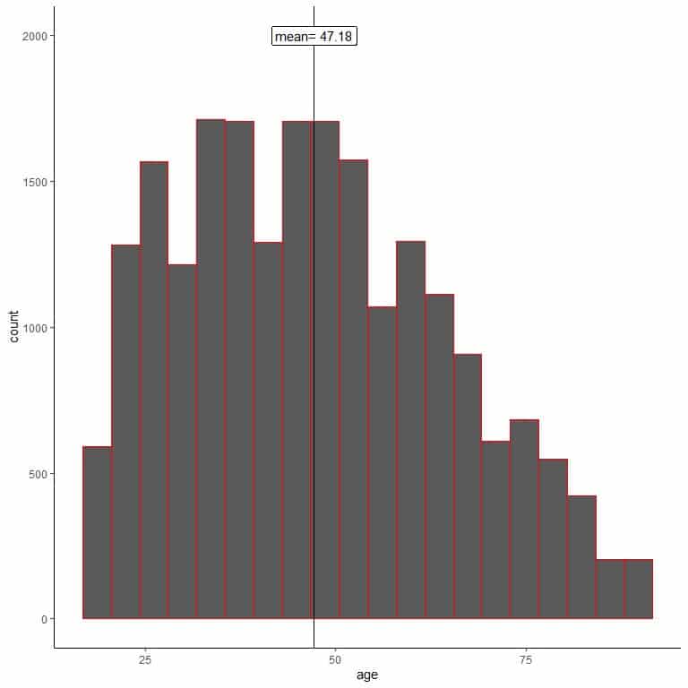
The population mean = 47.18 years, and the population distribution is slightly right-skewed.

One researcher uses random sampling to sample 200 individuals from this population.

In random sampling, the sample characteristics mimic those of the population. We can see that from the histogram of ages for his sample.

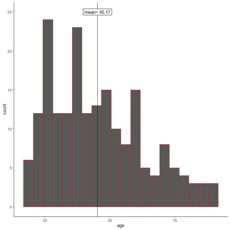
We see that the sample histogram is similar to that of the population (slightly right-skewed). Also, the sample mean = 45.17 years is a good approximation (estimate) to the true population mean = 47.18 years.

Another researcher does not use random sampling and sample 200 from his colleagues.

Let’s plot a histogram of his sample’s ages.

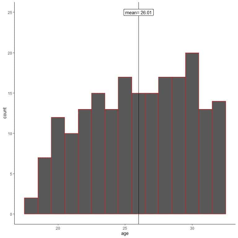
We see that the sample histogram is different from the population histogram. The sample histogram is slightly left-skewed, and not right skewed as population data.

Also, the sample mean = 26.01 years away from the true population mean = 47.18 years. The sample mean is a biased estimate of the population mean.

Sampling from his colleagues only has biased the sample mean to lower age value.

Sample mean formula

The sample mean formula is:

¯x=1/n ∑_(i=1)^n▒x_i

Where ¯x is the sample mean.

n is the sample size.

∑_(i=1)^n▒x_i means sum every element of our sample from x_1 to x_n.

Our sample element is denoted as x with a subscript to indicate its position in our sample.

In example 1, we have 20 ages, the first age (70) is denoted as x_1, the second age (56) is denoted as x_2, the third age (37) is denoted as x_3.

The last age (70) is denoted as x_20 or x_n because n = 20 in this case.

We used this formula in all the above examples. We summed the sample data and divided it by the sample size (or multiplied by 1/n).

Properties of the sample mean

Any sample we get randomly from a population is one of many possible samples that we may obtain by chance. The sample means based on a certain size vary across different samples of the same size.

– Example 1

For describing the distribution of age in a certain population, there are 3 groups of researchers:

1. Group 1 takes a sample of 100 individuals and gets a mean= 46.77 years.
2. Group 2 takes a sample of another 100 individuals and gets a mean= 47.44 years.
3. Group 3 takes a sample of another 100 individuals and gets a mean= 49.21 years.

We note that the sample means reported by the 3 groups are not identical, although they sampled the same population.

This variability in sample means will decrease by increasing the sample size; if these groups have taken samples of 1000 individuals, the variability observed between the 3 different 1000-sample means will be less than 100-sample.

– Example 2

For a certain population of more than 20,000 individuals, the true population mean for age in this population = 47.18 years.

Using the census data and a computer program:

1. We will generate 100 random samples, each of size 20, and calculate each sample’s mean. Then, we plot the sample means as histograms and dot plots to see their distribution.

means_20 are 100 different means, each based on a sample of size 20.

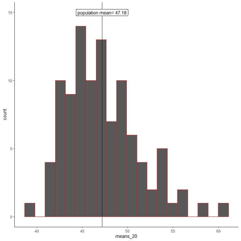
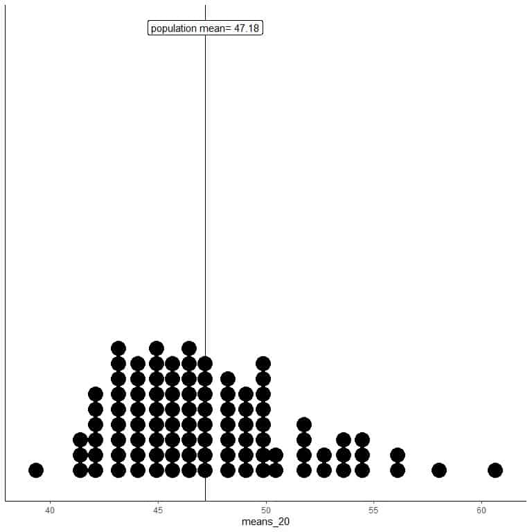
The range of means_20 (based on 20 sample size) is from nearly 40 to 60, and more means are clustered on the true population mean.

2. We will generate 100 random samples, each of size 100, and calculate the mean for each sample. Then, we plot the sample means as histograms and dot plots to see their distribution.

means_100 are 100 different means, each based on a sample of size 100.

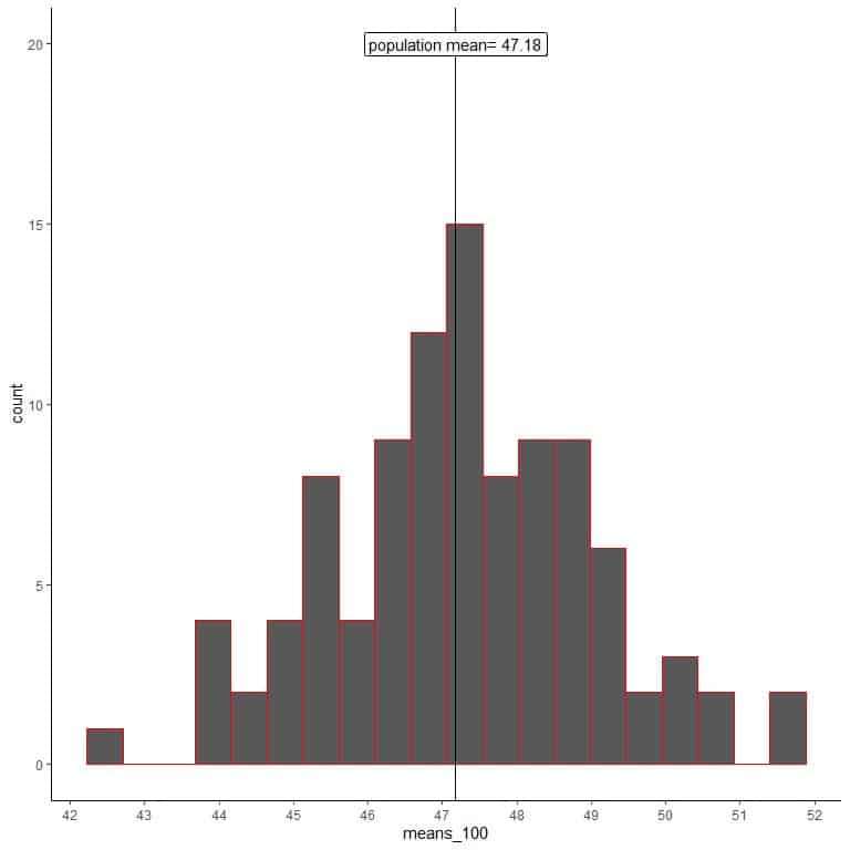
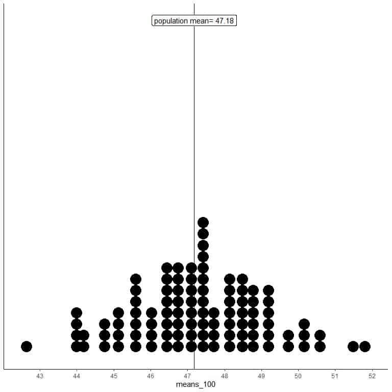
The range of means_100 (based on 100 sample size) is from nearly 43 to 52 and is narrower than that for means_20.

More means of means_100 are clustered on the true population mean than from means_20.

3. We will generate 100 random samples, each of size 1000, and calculate each sample’s mean. Then, we plot the sample means as histograms and dot plots to see their distribution.

means_1000 are 100 different means, each based on a sample of size 1000.

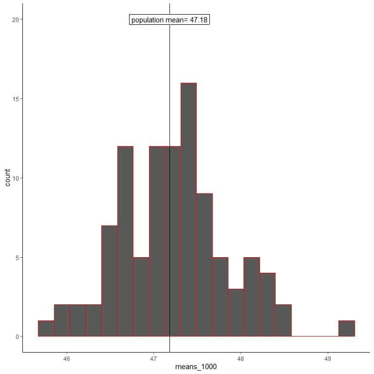
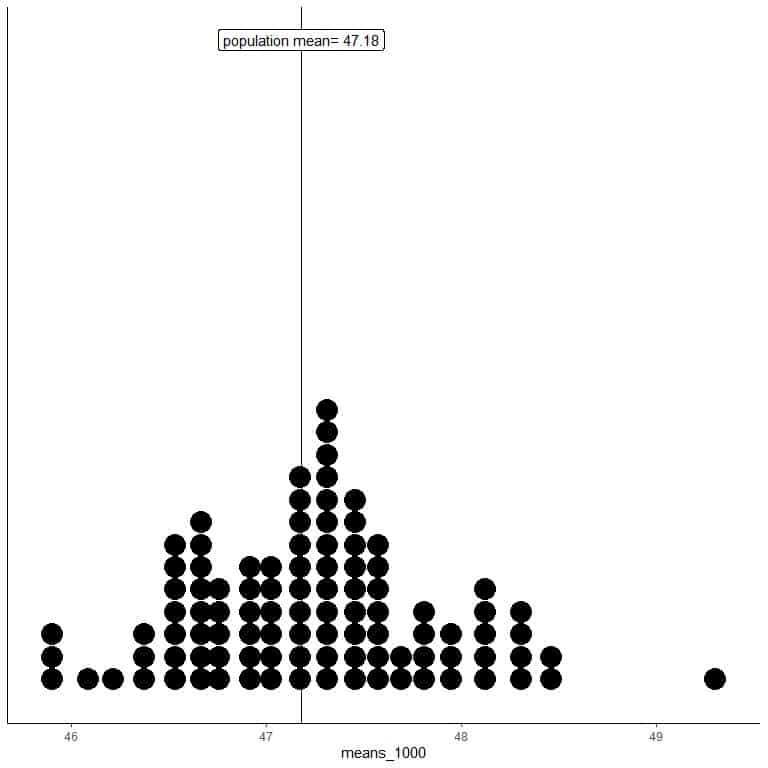The range of means_1000 (based on 1000 sample size) is from nearly 46 to 50 and is narrower than that for means_20 or means_100.

More means of means_1000 are clustered on the true population mean than from means_20 or means_100.

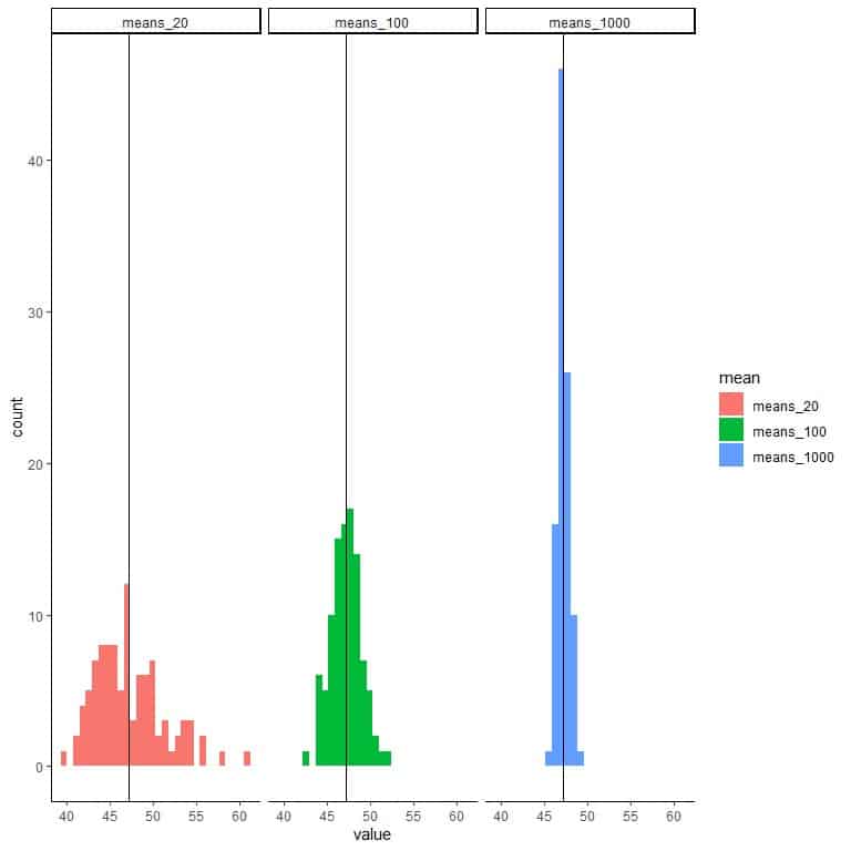
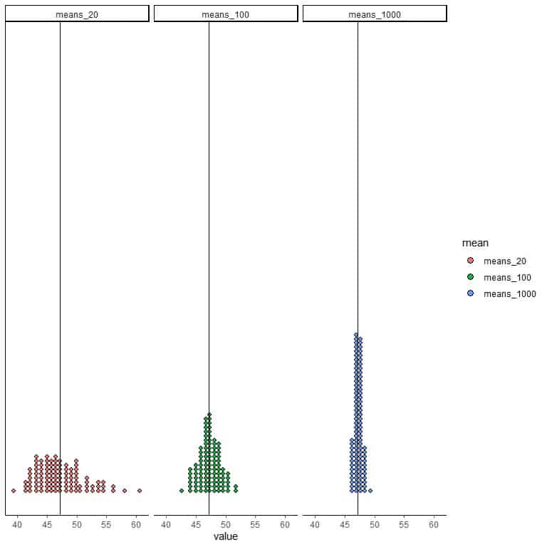
Plot all graphs side by side with a vertical line for the population mean.

Conclusions

1. The variation in the sample means decreases with increasing the sample size.
   More sample means will cluster on the true population mean with increasing sample size or become more precise.
2. In real-life research, only one sample is taken with a certain size from a specific population. With increasing the sample size, the sample mean is getting closer to the true population mean that we cannot measure.
3. The following table shows how many means from each group have a value between 47-48, so it is very close to the true population mean (47.18).

For means_1000 (based on 1000 sample size), 53 means out of 100 means are between 47-48.

For means_20 (based on 20 sample size), only 8 means out of 100 means are between 47-48.

Practice questions

1. We want to study the systolic blood pressure of some hypertensive patients. Because of limited resources, only 15 individuals are surveyed, and we have their systolic blood pressure in mmHg. What is the mean of this sample?
120 158 114 195 146 184 132 147 140 139 150 142 134 126 138.

2. The following are the body mass indices of a sample of 33 individuals from a certain population. What is the mean of this sample?

29.45 28.35 27.99 32.87 25.35 29.07 30.63 40.27 31.91 27.34 34.53 25.65 27.89 30.90 27.18 28.76 34.63 30.78 35.20 32.98 26.29 32.04 26.35 39.54 31.48 22.49 37.80 29.76 30.42 27.30 27.01 29.02 43.85.

3. The following are the air pressure at the storm’s center (in millibars) of a sample of 30 storms from a certain dataset. What is the mean of this sample?

1013 1013 1013 1013 1012 1012 1011 1006 1004 1002 1000 998 998 998 987 987 984 984 984 984 984 984 981 986 986 986 986 986 986 986.

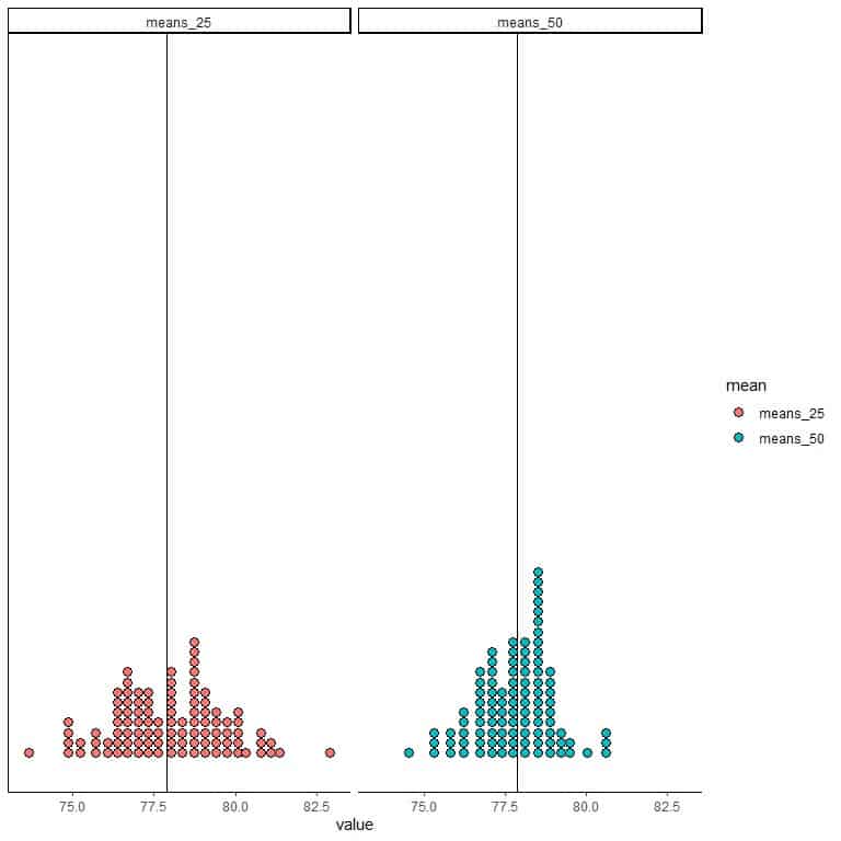
4. The following are dot plots for 2 groups of 100 sample means. One group is based on 25 sample sizes (means_25), and the other group is based on 50 sample sizes (means_50). Which sample size has produced the most precise estimate of the true population mean?

The true population mean is indicated by the solid vertical line.

5. The following table is the minimum and maximum for 4 groups of 50 sample means. Each group is based on a different sample size. Which sample size has produced the most precise estimate of the true population mean?

Answer key

1.

• Sum of the numbers = 2165.
• The number of items in your sample = 15.
• Divide the first number by the second number to get the sample mean.

The sample mean = 2165/15 = 144.33 mmHg.

2.

• Sum of the numbers = 1015.08.
• The number of items in your sample = 33.
• Divide the first number by the second number to get the sample mean.

The sample mean = 1015.08/33 = 30.76.

3.

• Sum of the numbers = 29854.
• The number of items in your sample = 30.
• Divide the first number by the second number to get the sample mean.

The sample mean = 29854/30 = 995.13 millibars.

4. Sample size = 50 because more means are clustered around the true population mean than that observed for sample size = 25.

5. We see that samples based on size = 800 have the lowest range (from 51 to 56), so it is the most precise estimate.

Previous Lesson | Main Page | Next Lesson