The Sample Variance – Explanation & Examples

The definition of the sample variance is:

“The sample variance is the average of the squared differences from the mean found in a sample.”

In this topic, we will discuss the sample variance from the following aspects:

• What is the sample variance?
• How to find the sample variance?
• Sample variance formula.
• The role of the sample variance.
• Practice questions.
• Answer key.

What is the sample variance?

The sample variance is the average of the squared differences from the mean found in a sample.

The sample variance measures the spread of a numerical characteristic of your sample.

A large variance indicates that your sample numbers are far from the mean and far from each other.

A small variance, on the other hand, indicates the opposite.

A zero variance indicates that all values within your sample are identical.

The variance can be zero or a positive number. Still, it cannot be negative because it is mathematically impossible to have a negative value resulting from a square.

For example, if you have two sets of 3 numbers (1,2,3) and (1,2,10). You see that the second set is more spread (more varied) than the first set.

You can see that from the following dot plot.

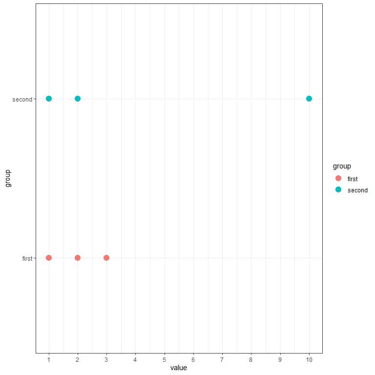
We see that the blue dots (second group) are more spread out than the red dots (first group).

If we calculate the first group variance, it is 1, while the variance for the second group is 24.3. Therefore, the second group is more spread (more varied) than the first group.

How to find the sample variance?

We will go through several examples, from simple to more complex ones.

– Example 1

What is the variance of the numbers, 1,2,3?

1. Add up all of the numbers:

1+2+3 = 6.

2. Count the numbers of items in your sample. In this sample, there are 3 items.

3. Divide the number you found in step 1 by the number you found in step 2.

The sample mean = 6/3 = 2.

4. In a table, subtract the mean from each value of your sample.

You have a table of 2 columns, one for the data values and the other column for subtracting the mean (2) from each value.

4. Add another column for the squared differences you found in Step 4.

6. Add up all of the squared differences you found in Step 5.

1+0+1 = 2.

7. Divide the number you get in step 6 by sample size-1 to get the variance. We have 3 numbers, so the sample size is 3.

The variance = 2/(3-1) = 1.

– Example 2

What is the variance of the numbers, 1,2,10?

1. Add up all of the numbers:

1+2+10 = 13.

2. Count the numbers of items in your sample. In this sample, there are 3 items.

3. Divide the number you found in step 1 by the number you found in step 2.

The sample mean = 13/3 = 4.33.

4. In a table, subtract the mean from each value of your sample.

You have a table of 2 columns, one for the data values and the other column for subtracting the mean (4.33) from each value.

5. Add another column for the squared differences you found in Step 4.

6. Add up all of the squared differences you found in Step 5.

11.09 + 5.43 + 32.15 = 48.67.

7. Divide the number you get in step 6 by sample size-1 to get the variance. We have 3 numbers, so the sample size is 3.

The variance = 48.67/(3-1) = 24.335.

– Example 3

The following is the age (in years) of 25 individuals sampled from a certain population. What is the variance of this sample?

1. Add up all of the numbers:

26+ 48+ 67+ 39+ 25+ 25+ 36+ 44+ 44+ 47+ 53+ 52+ 52+ 51+ 52+ 40+ 77+ 44+ 40+ 45+ 48+ 49+ 19+ 54+ 82 = 1159.

2. Count the numbers of items in your sample. In this sample, there are 25 items or 25 individuals.

3. Divide the number you found in step 1 by the number you found in step 2.

The sample mean = 1159/25 = 46.36 years.

4. In a table, subtract the mean from each value of your sample.

There is one column for the ages and another column for subtracting the mean (46.36) from each value.

5. Add another column for the squared differences you found in Step 4.

6. Add up all of the squared differences you found in Step 5.

414.53+ 2.69+ 426.01+ 54.17+ 456.25+ 456.25+ 107.33+ 5.57+ 5.57+ 0.41+ 44.09+ 31.81+ 31.81+ 21.53+ 31.81+ 40.45+ 938.81+ 5.57+ 40.45+ 1.85+ 2.69+ 6.97+ 748.57+ 58.37+ 1270.21 = 5203.77.

7. Divide the number you get in step 6 by sample size-1 to get the variance. We have 25 numbers so the sample size is 25.

The variance = 5203.77/(25-1) = 216.82 years^2.

Note that the sample variance has the squared unit of the original data (years^2) due to the presence of squared difference in its calculation.

– Example 4

The following is the score (in points) of 10 students in an easy exam. What is the variance of this sample?

All students have 100 points on this exam.

1. Add up all of the numbers:

Sum = 1000.

2. Count the numbers of items in your sample. In this sample, there are 10 items or students.

3. Divide the number you found in step 1 by the number you found in step 2.

The sample mean = 1000/10 = 100.

4. In a table, subtract the mean from each value of your sample.

5. Add another column for the squared differences you found in Step 4.

6. Add up all of the squared differences you found in Step 5.

Sum = 0.

7. Divide the number you get in step 6 by sample size-1 to get the variance. We have 10 numbers, so the sample size is 10.

The variance = 0/(10-1) = 0 points^2.

The variance can be zero if all our sample values are identical.

– Example 5

The following table shows the daily closing prices (in US dollars or USD) of Facebook (FB) and Google (GOOG) stocks in some days of 2013. Which stock has a more variable closing stock price?

Note that we compare the two stocks from the same sector (communication services) and for the same period.

We will calculate the variance for each stock then compare between them.

The variance of Facebook stock closing price is calculated as follows:

1. Add up all of the numbers:

28.00+ 27.77+ 28.76+ 29.42+ 29.06+ 30.59+ 31.30+ 31.72+ 30.95+ 30.10+ 29.85+ 30.14+ 29.66+ 30.73+ 30.82+ 31.08+ 31.54+ 32.47+ 30.79+ 31.24+ 30.98+ 29.73+ 28.11+ 28.64+ 29.05+ 28.65+ 28.55+ 28.26+ 27.37+ 27.91+ 28.50+ 28.32+ 28.93+ 28.46+ 27.28+ 27.13+ 27.27+ 27.39+ 26.87+ 27.25+ 27.78+ 27.72+ 27.52+ 27.45+ 28.58+ 27.96+ 28.14+ 27.83+ 27.08+ 27.04 = 1447.74.

2. Count the numbers of items in your sample. In this sample, there are 50 items.

3. Divide the number you found in step 1 by the number you found in step 2.

The sample mean = 1447.74/50 = 28.9548 USD.

4. In a table, subtract the mean from each value of your sample.

There is one column for the stock prices and another column for subtracting the mean (28.9548) from each value.

5. Add another column for the squared differences you found in Step 4.

6. Add up all of the squared differences you found in Step 5.

0.91+ 1.40+ 0.04+ 0.22+ 0.01+ 2.67+ 5.50+ 7.65+ 3.98+ 1.31+ 0.80+ 1.40+ 0.50+ 3.15+ 3.48+ 4.52+ 6.68+ 12.36+ 3.37+ 5.22+ 4.10+ 0.60+ 0.71+ 0.10+ 0.01+ 0.09+ 0.16+ 0.48+ 2.51+ 1.09+ 0.21+ 0.40+ 0.00+ 0.24+ 2.80+ 3.33+ 2.84+ 2.45+ 4.35+ 2.91+ 1.38+ 1.52+ 2.06+ 2.26+ 0.14+ 0.99+ 0.66+ 1.27+ 3.51+ 3.67 = 112.01.

7. Divide the number you get in step 6 by sample size-1 to get the variance. We have 50 numbers so the sample size is 50.

8. The variance of Facebook stock closing price = 112.01/(50-1) = 2.29 USD^2.

The variance of Google stock closing price is calculated as follows:

1. Add up all of the numbers:

723.2512+ 723.6713+ 737.9713+ 734.7513+ 733.3012+ 738.1212+ 741.4813+ 739.9913+ 723.2512+ 724.9313+ 715.1912+ 711.3212+ 704.5112+ 702.8712+ 741.5013+ 754.2113+ 753.6713+ 750.7313+ 753.6813+ 753.8313+ 755.6913+ 775.6013+ 759.0213+ 765.7413+ 770.1713+ 773.9513+ 785.3714+ 782.4213+ 780.7013+ 782.8613+ 787.8214+ 792.8913+ 806.8514+ 792.4613+ 795.5313+ 799.7114+ 790.7714+ 790.1313+ 799.7813+ 801.2014+ 806.1914+ 821.5014+ 838.6014+ 831.3814+ 832.6014+ 831.5214+ 834.8214+ 827.6114+ 825.3114+ 821.5414 = 38622.02.

2. Count the numbers of items in your sample. In this sample, there are 50 items.

3. Divide the number you found in step 1 by the number you found in step 2.

The sample mean = 38622.02/50 = 772.4404 USD.

4. In a table, subtract the mean from each value of your sample.

There is one column for the stock prices and another column for subtracting the mean (772.4404) from each value.

5. Add another column for the squared differences you found in Step 4.

6. Add up all of the squared differences you found in Step 5.

2419.58+ 2378.43+ 1188.12+ 1420.47+ 1531.88+ 1177.81+ 958.47+ 1052.94+ 2419.58+ 2257.11+ 3277.47+ 3735.56+ 4614.38+ 4839.87+ 957.23+ 332.30+ 352.28+ 471.29+ 351.90+ 346.30+ 280.53+ 9.99+ 180.07+ 44.88+ 5.15+ 2.28+ 167.21+ 99.62+ 68.24+ 108.60+ 236.58+ 418.24+ 1184.12+ 400.84+ 533.19+ 743.71+ 336.03+ 312.97+ 747.52+ 827.20+ 1139.13+ 2406.98+ 4377.28+ 3474.04+ 3619.35+ 3490.56+ 3891.39+ 3043.84+ 2795.34+ 2410.91 = 73438.76.

7. Divide the number you get in step 6 by sample size-1 to get the variance. We have 50 numbers, so the sample size is 50.

The Google stock closing price variance = 73438.76/(50-1) = 1498.75 USD^2, while the variance of the Facebook stock closing price is 2.29 USD^2.

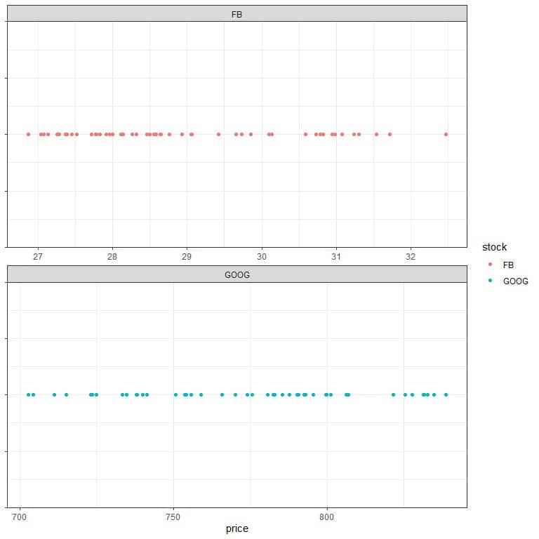
The Google stock closing price is more variable. We can see that if we plot the data as a dot plot.

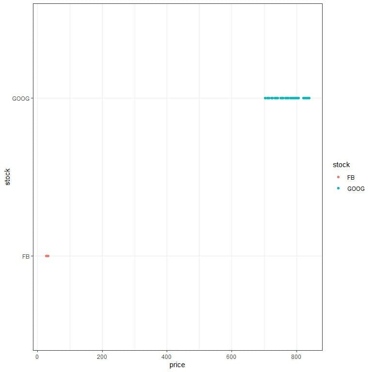
In the first plot, when the x-axis is common, we see that the Facebook prices occupy a small space compared to Google prices.

In the second plot, when the x-axis values are set according to each stock’s values, we see that Facebook prices range from 27 to 32, while Google prices range from 700 to about 850.

Sample variance formula

The sample variance formula is:

s^2=(∑_(i=1)^n▒( x_i-¯x )^2)/(n-1)

Where s^2 is the sample variance.

¯x is the sample mean.

n is the sample size.

The term:

∑_(i=1)^n▒( x_i-¯x )^2

means sum the squared difference between every element of our sample (from x_1 to x_n) and the sample mean ¯x.

Our sample element is denoted as x with a subscript to indicate its position in our sample.

In the example of stock prices for Facebook, we have 50 prices. The first price (28) is denoted as x_1, the second price (27.77) is denoted as x_2, the third price (28.76) is denoted as x_3.

The last price (27.04) is denoted as x_50 or x_n because n = 50 in this case.

We used this formula in the above examples, where we summed the squared difference between every element of our sample and the sample mean, then divided by the sample size-1 or n-1.

We divide by n-1 when calculating the sample variance (and not by n as any average) to make the sample variance a good estimator of the true population variance.

If you have population data, you will divide by N (where N is the population size) to get the variance.

– Example

We have a population of more than 20,000 individuals. From the census data, the true population variance for the age was 298.84 years^2.

We take a random sample of 50 individuals from this data. The sum of squared differences from the mean was 12112.08.

If we divide by 50 (sample size), the variance will be 242.24, while if we divide by 49 (sample size-1), the variance will be 247.19.

Dividing by n-1 prevents the sample variance from underestimating the true population variance.

The role of the sample variance

The sample variance is a summary statistic that can be used to deduce the spread of the population from which the sample was randomly selected.

In the above example about Google and Facebook stock prices, although we have only a sample of 50 days, we can conclude (with some level of certainty) Google stock is more variable (riskier) than Facebook stock.

Variance is important in an investment where we can use it (as a measure of spread or variability) as a measure of risk.

We see in the above example that although Google stock has a higher closing price, it is more variable and so more risky to invest in.

Another example is when the product produced from some machines is with high variance in the industrial machines. It indicates that these machines need adjustment.

Disadvantages of variance as a measure of spread:

1. It is affected by outliers. These are the numbers that are far from the mean. Squaring the differences between these numbers and the mean can skew the variance.
2. Not easily interpreted because the variance has the squared unit of the data.

We use the variance to take the square root of its value, which indicates the standard deviation of the data set. Thus, the standard deviation has the same unit as the original data, so it is more easily interpreted.

Practice questions

1. The following table is the daily closing prices (in USD) of two stocks from the financial sector, JP Morgan Chase (JPM) and Citigroup (C), for some days in 2011. Which stock has a more variable closing stock price?

2. The following is a table of the compressive strengths for 25 concrete samples (in pound per square inch or psi) produced from 3 different machines. Which machine is more precise in its production?

Note more precise means less variable.

3. The following is a table for the variance in weights of diamonds produced from 4 different machines and a dot plot for the individual weight values.

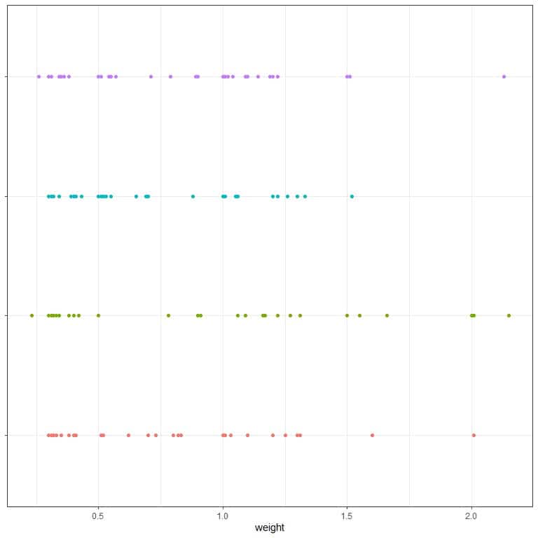We see that machine_3 has the least variance. Knowing that, which dots are most likely produced from machine_3?

4. The following is the variance for different stocks closing prices (from the same sector). Which stock is safer to invest in?

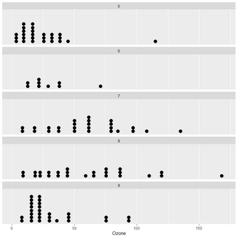
5. The following dot plot is for the daily Ozone measurements in New York, May to September 1973. Which month is the most variable in Ozone measurements, and which month is the least variable?

Answer key

1. We will calculate the variance for each stock then compare between them.

The variance of JP Morgan Chase stock closing price is calculated as follows:

• Add up all of the numbers:

Sum = 1219.85.

• Count the numbers of items in your sample. In this sample, there are 30 items.
• Divide the number you found in step 1 by the number you found in step 2.

The sample mean = 1219.85/30 = 40.66167.

• Subtract the mean from each value of your sample and square the difference.

• Add up all of the squared differences you found in Step 4.

Sum = 14.77.

• Divide the number you get in step 5 by sample size-1 to get the variance. We have 30 numbers, so the sample size is 30.

The variance of JPM stock closing price = 14.77/(30-1) = 0.51 USD^2.

The variance of Citigroup stock closing price is calculated as follows:

• Add up all of the numbers:

Sum = 1189.25.

• Count the numbers of items in your sample. In this sample, there are 30 items.
• Divide the number you found in step 1 by the number you found in step 2.

Тhe sample mean = 1189.25/30 = 39.64167.

• Subtract the mean from each value of your sample and square the difference.

• Add up all of the squared differences you found in step 4.

Sum = 80.77.

• Divide the number you get in step 5 by sample size-1 to get the variance. We have 30 numbers, so the sample size is 30.

Citigroup stock closing price variance = 80.77/(30-1) = 2.79 USD^2, while the variance of JP Morgan Chase stock closing price is only 0.51 USD^2.

The Citigroup stock closing price is more variable. We can see that if we plot the data as a dot plot.

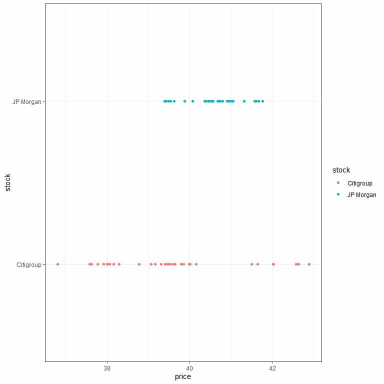
When the x-axis is common, we see that the Citigroup prices are more scattered than JP Morgan prices.

2. We will calculate the variance for each machine then compare them.

The variance of machine_1 is calculated as follows:

•  Add up all of the numbers:

Sum = 888.45.

• Count the numbers of items in your sample. In this sample, there are 25 items.
• Divide the number you found in step 1 by the number you found in step 2.

The sample mean = 888.45/25 = 35.538.

• Subtract the mean from each value of your sample and square the difference.

• Add up all of the squared differences you found in Step 4.

Sum = 5735.17.

• Divide the number you get in step 5 by sample size-1 to get the variance. We have 25 numbers, so the sample size is 25.

The variance of machine_1 = 5735.17/(25-1) = 238.965 psi^2.

With similar calculations, the variance of machine_2 = 315.6805 psi^2, and the variance for machine_3 = 310.7079 psi^2.

The machine_1 is more precise or less variable in the compressive strength of concrete produced.

3. Blue dots because they are more compact than other dot groups.

4. Stock_2 because it has the least variance.

5. The most variable month is 8 or August and the least variable month is 6 or June.

Previous Lesson | Main Page | Next Lesson