Sampling Distribution – Explanation & Examples

The definition of a sampling distribution is:

“The sampling distribution is a probability distribution of a statistic obtained from a larger number of samples with the same size and randomly drawn from a specific population.”

In this topic, we will discuss the sampling distribution from the following aspects:

1. What is the sampling distribution?
2. Sampling distribution formula for the mean.
3. How to calculate the sampling distribution for the mean?
4. Sampling distribution formula for proportion.
5. How to calculate the sampling distribution for proportion?
6. Practice questions.
7. Answer key.

1. What is the sampling distribution?

The sampling distribution is a theoretical distribution, that we cannot observe, that describes all the possible values of a sample statistic (like mean or proportion) from random samples of the same size that are taken from the same population.

In real-life research, only one sample is taken with a certain size from a specific population. This sample is one of many possible samples that we may get by chance.

There are many types of sample statistics that we can estimate from our samples:

• The sample mean for continuous variables.
• The sample proportion for categorical variables.
• The sample mean difference for comparing 2 continuous variables.
• The sample proportion difference for comparing 2 categorical variables.

These sample statistics vary across different samples of the same size. This variability in sample statistics is called the standard error (SE) and is different from the variability of individual values in any single sample, which is called the standard deviation (s).

– Example of the sampling distribution for the sample mean

We have population data for individual body mass index (bmi). We know that the population mean for these body mass indices is 29.97.

The distribution of bmi in this population is normal or bell-shaped as we see from the histogram below.

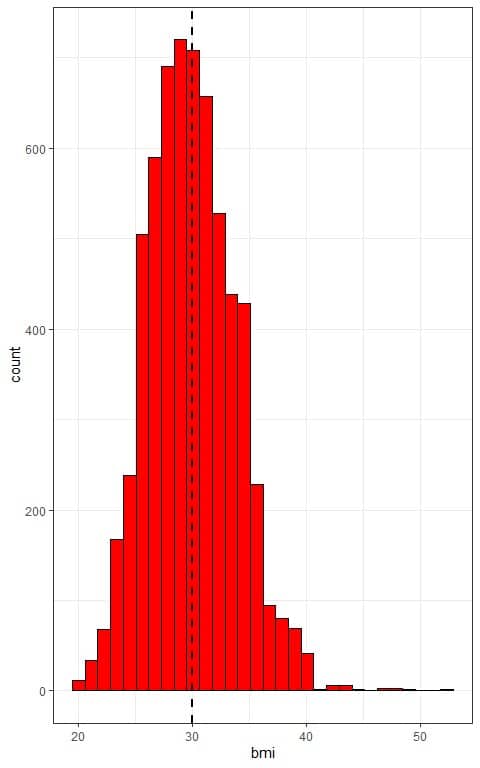
The x-axis is the individual bmi values and the histogram has a normally distributed shape that is symmetric around the population mean (plotted as a vertical dashed line).

Using a computer program, we will take 1000 random samples from this population data, each of size 30, 100, or 200, calculate the sample mean for each sample, and plot the samples’ means as histograms to see their (sampling) distribution.

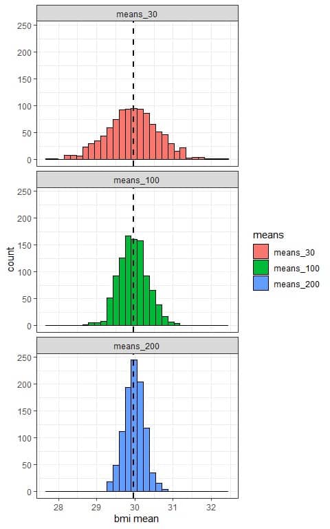
We see that:

• The x-axis is the mean value from each sample.
• We have 3 histograms, one for the sample means based on 30 sample size (means_30), one for the sample means based on 100 sample size (means_100), and the last one for the sample means based on 200 sample size (means_200).
• The (sampling) distribution of sample means is normally distributed (bell-shaped) for all sample sizes (30, 100, and 200), and centered around the population mean which is plotted as a black dashed line.
• The variability of the sampling distribution for the sample means decreases with increasing the sample size.

The following table lists the mean and standard deviation (or standard error) of each 1000 sample means:

We see that:

• The mean of each 1000 sample means based on size 30, 100, or 200 is nearly equal to the true population mean (29.97).
• The standard deviation (or standard error SE) of the 1000 sample means decreases with increasing the sample size.

– Example of the sampling distribution for sample means from skewed data

We have population data for individual physical activity (Kcal/week). We know that the population mean for these physical activities is 398.83 Kcal/week.

The distribution of physical activity in this population is right-skewed as we see from the histogram below.

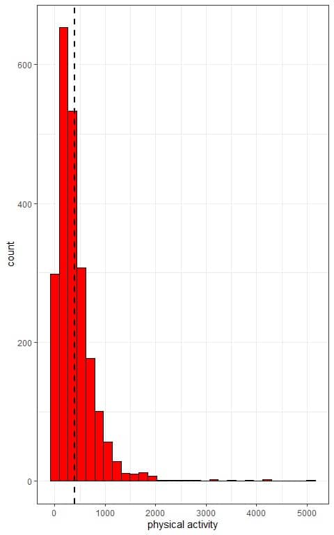
The x-axis is the individual physical activity values and the histogram has a right-skewed shape with low frequent large values.

The histogram is not symmetric around the population mean (plotted as a vertical dashed line).

Using a computer program, we will take 1000 random samples from this population data, each of size 30, 100, or 200, calculate the sample mean for each sample, and plot the samples’ means as histograms to see their (sampling) distribution.

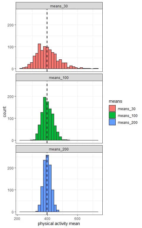
We see that:

• The x-axis is the mean value from each sample.
• We have 3 histograms, one for the sample means based on 30 sample size (means_30), one for the sample means based on 100 sample size (means_100), and the last one for the sample means based on 200 sample size (means_200).
• The (sampling) distribution of sample means is normally distributed (bell-shaped) for all sample sizes (30, 100, and 200), and centered around the population mean which is plotted as a black dashed line.
• The variability of the sampling distribution for the sample means decreases with increasing the sample size.

The following table lists the mean and standard deviation (or standard error) of each 1000 sample means:

We see that:

• The mean of each 1000 sample means based on size 30, 100, or 200 is nearly equal to the true population mean (398.83).
• The standard deviation (or standard error SE) of the 1000 sample means decreases with increasing the sample size.

– Example of the sampling distribution for sample proportions

We have population data for individual ethnicities. We know that the true population proportion for White persons is 0.763 or 76.3%.

We can see the percentage of White and non-White individuals from the following bar plot.

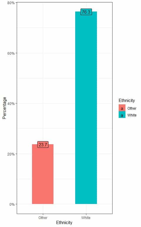
We see that the percentage of White individuals is 76.3% and the percentage of Other individuals is 23.7%.

Using a computer program, we will take 1000 random samples from this population data, each of size 50, 100, or 200, calculate the White proportion from each sample, and plot the different sample proportions as histograms to see their sampling distribution.

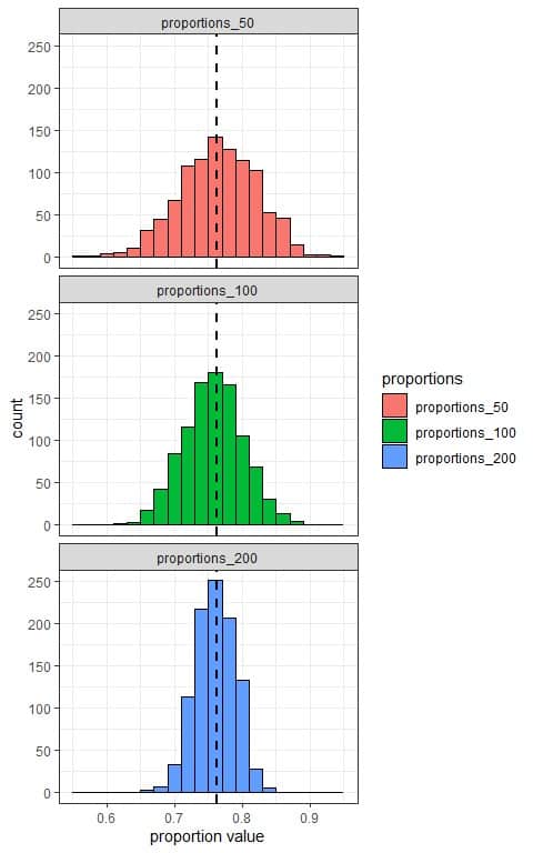
We see that:

• The x-axis is the proportion value from each sample.
• We have 3 histograms, one for the sample proportions based on 50 sample size (proportions_50), one for the sample proportions based on 100 sample size (proportions_100), and the last one for the sample proportions based on 200 sample size (proportions_200).
• The (sampling) distribution of sample proportions is normally distributed (bell-shaped) for all sample sizes (50, 100, and 200), and centered around the population proportion which is plotted as a black dashed line.
• The variability of the sampling distribution for the sample proportions decreases with increasing the sample size.

The following table lists the mean and standard deviation (or standard error) of each 1000 sample proportions:

We see that:

• The mean of each 1000 sample proportions based on size 50, 100, or 200 is nearly equal to the true population proportion (0.763).
• The standard deviation (or standard error SE) of the 1000 sample proportions decreases with increasing the sample size.

The reason for the decrease in the variability of the distribution with increasing the sample size is that the sample estimates (means or proportions) will be less affected by sample data (individual observations) with increasing the sample size.

– Sampling distribution formula for the mean

For a large sample of size n ≥ 30 independent observations, the sampling distribution of the sample mean ¯x will be nearly normal with:

μ_¯x=μ

and

SE=σ/√n

Where:

μ_¯x is the mean of the sample means with the same size (n).

μ is the population mean.

SE is the standard error or the variability in the sample means.

σ is the population standard deviation. It can be replaced by the sample standard deviation (s) when the sample size is ≥ 30.

2. How to calculate the sampling distribution for the mean?

We use the rules of the normal distribution to define the sampling distribution for a sample mean.

For any normal distribution, 95% of the data are within 1.96 standard deviations from the mean and 99% of the data are within 2.58 standard deviations from the mean.

We follow these steps:

1. Check for the needed sample conditions so that the sampling distribution of its mean is normal:

• The data must be independent.
• The data should be of size ≥ 30.

2. Calculate the sample mean ¯x and the sample standard deviation (s).

3. Use the sample standard deviation to calculate the standard error SE.

4. Use the sample mean as an estimate of the population mean μ and the SE to construct 95% and 99% confidence intervals that most likely contains the population mean.

95% confidence interval = ¯x±1.96XSE = ¯x±1.96X s/√n.

99% confidence interval = ¯x±2.58XSE = ¯x±2.58X s/√n.

– Interpretation of confidence intervals

A confidence interval gives us a range of possible values for the unknown population parameter (mean or proportion) from which the sample was taken.

The 95% confidence interval from a sample with a certain size means that, for 95% of samples taken from this population and with the same size, the confidence interval 4generated from them will contain the true population parameter.

The 99% confidence interval from a sample with a certain size means that, for 99% of samples taken from this population and with the same size, the confidence interval generated from them will contain the true population parameter.

As long as the 95% confidence interval works 95% of the time, we are 95% confident that the constructed interval contains the population value.

As long as the 99% confidence interval works 99% of the time, we are 99% confident that the constructed interval contains the population value.

The 99% confidence interval will be wider than the 95% confidence interval which we will see in the following example.

– Example 1

The following is the waist circumference (in mm) of 30 individuals randomly sampled from a certain population.

What is the 95% and 99% confidence interval for the mean waist circumference of this population?

1. Check for the needed sample conditions so that the sampling distribution of its mean is normal:

• The sample data must be independent. The data are randomly sampled from the population so they are independent.
• The sample should be of size ≥ 30 which is also true.

2. Calculate the sample mean ¯x and the sample standard deviation (s).

• Add up all of the data, sum = 3036.
• Divide the sum of your data by the count of your data to get the sample mean.

The sample mean = 3036/30 = 101.2 mm.

• In a table, subtract the mean from each value of your sample.

• Add another column for the squared differences.

• Add up all of the squared differences, the sum = 3626.8.
• Divide the sum of squared differences sample size-1 to get the variance.

The variance = 3626.8/(30-1) = 125.0621 mm^2.

• Take the square root of the variance to get the standard deviation.

The standard deviation = √125.621 = 11.18 mm.

3. Use the sample standard deviation (s) to calculate the standard error SE.

SE=s/√n=11.18/√30 = 2.04.

4. Use the sample mean as an estimate of the population mean μ and the SE to construct 95% and 99% confidence intervals that most likely contains the population mean.

95% confidence interval = ¯x±1.96XSE = 101.2-1.96X2.04 to 101.2+1.96X2.04 = 97.20 to 105.20.

We are 95% confident that the true population mean waist circumference is between 97.20 and 105.20 mm.

99% confidence interval = ¯x±2.58XSE = 101.2-2.58X2.04 to 101.2+2.58X2.04 = 95.94 to 106.46.

We are 99% confident that the true population mean waist circumference is between 95.94 and 106.46 mm.

– Example 2

The following table shows the mean and standard deviation of the weights of 50, 100, and 200 diamonds randomly sampled from a population of about 54,000 diamonds.

What is the 95% and 99% confidence interval for the mean weight of this population from each sample?

1. Check for the needed sample conditions so that the sampling distribution of its mean is normal:

• The sample data must be independent. The data are randomly sampled from the population so they are independent.
• The sample should be of size ≥ 30 which is also true.

2. Calculate the sample mean ¯x and the sample standard deviation (s).

• Each sample has its mean and standard deviation shown in the above table.

3. Use the sample standard deviation (s) to calculate the standard error SE.

For sample size 50, SE=s/√n=0.47/√50 = 0.066.

For sample size 100, SE=s/√n=0.51/√100 = 0.051.

For sample size 200, SE=s/√n=0.42/√200 = 0.03.

Note that the SE decreases with increasing the sample size.

We update the table to add a column for the SE.

4. Use the sample mean as an estimate of the population mean μ and the SE to construct 95% and 99% confidence intervals that most likely contains the population mean.

For sample size 50, 95% confidence interval = ¯x±1.96XSE = 0.82-1.96X0.066 to 0.82+1.96X0.066 = 0.691 to 0.949.

For sample size 50, 99% confidence interval = ¯x±2.58XSE = 0.82-2.58X0.066 to 0.82+2.58X0.066 = 0.650 to 0.99.

For sample size 100, 95% confidence interval = ¯x±1.96XSE = 0.84-1.96X0.051 to 0.84+1.96X0.051 = 0.740 to 0.94.

For sample size 100, 99% confidence interval = ¯x±2.58XSE = 0.84-2.58X0.051 to 0.84+2.58X0.051 = 0.708 to 0.972.

For sample size 200, 95% confidence interval = ¯x±1.96XSE = 0.77-1.96X0.03 to 0.77+1.96X0.03 = 0.711 to 0.829.

For sample size 200, 99% confidence interval = ¯x±2.58XSE = 0.77-2.58X0.03 to 0.77+2.58X0.03 = 0.693 to 0.847.

We can update the table to added columns for different intervals.

We can plot the different confidence intervals according to the sample size in the following plot.

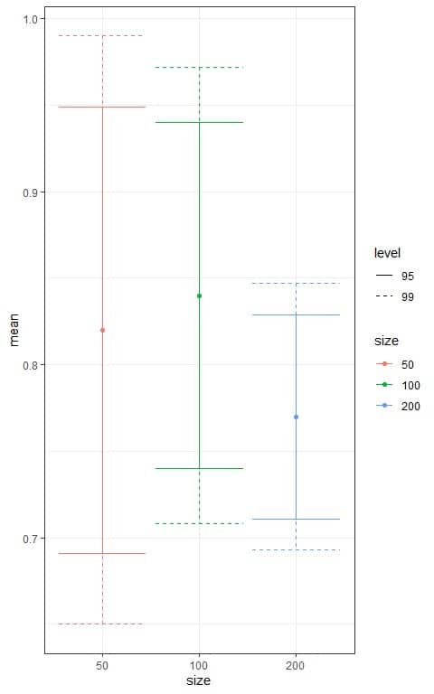
We see that:

• The confidence interval based on the 200 sample size is the narrowest interval.
• For each sample size, the 95% confidence interval (solid line) is tighter than the 99% confidence interval (dashed line).

4. Sampling distribution formula for proportion.

For a large sample of n independent observations so that np ≥ 10 and n(1-p) ≥ 10, the sampling distribution of the sample proportion p ̂ will be nearly normal with:

μ_p ̂ =p

and

SE=√((p(1-p))/n)

Where:

μ_p ̂ is the mean of the sample proportions with the same size (n).

p is the population proportion. It can be replaced by the sample proportion (p ̂) for calculating the standard error when np ̂≥10 and n(1-p ̂)≥10.

SE is the standard error or the variability in the sample proportions.

5. How to calculate the sampling distribution for proportion?

We use the rules of the normal distribution to define the sampling distribution for a sample proportion.

For any normal distribution, 95% of the data are within 1.96 standard deviations from the mean and 99% of the data are within 2.58 standard deviations from the mean.

We follow these steps:

1. Calculate the sample proportion p ̂.

2. Check for the needed sample conditions so that the sampling distribution of its proportion p ̂ is normal:

• The data must be independent.
• The np ̂≥10 and n(1-p ̂)≥10.

3. Use the sample proportion p ̂ to calculate the standard error SE.

4. Use the sample proportion p ̂ as an estimate of the population proportion p and the SE to construct a 95% and 99% confidence intervals that most likely contains the true population proportion.

95% confidence interval = p ̂±1.96XSE = p ̂±1.96X√((p(1-p))/n).

99% confidence interval = p ̂±2.58XSE = p ̂±2.58X√((p(1-p))/n).

– Example 1

The following data are the diabetic status of 50 randomly sampled persons from a certain population.

0 means healthy persons and 1 means diabetic persons.

0 1 0 1 1 0 0 1 0 0 1 0 0 0 0 1 0 0 0 1 1 0 0 1 0 1 0 0 0 0 1 1 0 1 0 0 1 0 0 0 0 0 0 0 0 0 0 0 0 1.

What are the 95% and 99% confidence intervals for the true diabetic proportion in this population?

We follow these steps:

1. Calculate the sample proportion p ̂.

By counting ones, we have 15 diabetic persons in our sample so:

The sample proportion p ̂ = 15/50 = 0.3.

2. Check for the needed sample conditions so that the sampling distribution of its proportion p ̂ is normal:

• The data must be independent.

The data are randomly sampled from a population so this condition is true.

• The np ̂≥10 and n(1-p ̂)≥10.

50 X 0.3 = 15 and 50 X (1-0.3) = 35. Both numbers are larger than 10 so this condition is true also.

3. Use the sample proportion p ̂ to calculate the standard error SE.

SE=√((p(1-p))/n)=√((0.3(1-0.3))/50)=0.065.

4. Use the sample proportion p ̂ as an estimate of the population proportion p and the SE to construct a 95% and 99% confidence intervals that most likely contains the true population proportion.

95% confidence interval = p ̂±1.96XSE = 0.3-1.96X0.065 to 0.3+1.96X0.065 = 0.173 to 0.427.

We are 95% confident that the true population proportion for diabetic persons is between 0.173 and 0.427 or between 17.3% and 42.7%.

99% confidence interval = p ̂±2.58XSE = 0.3-2.58X0.065 to 0.3+2.58X0.065 = 0.132 to 0.468.

We are 99% confident that the true population proportion for diabetic persons is between 0.132 and 0.468 or between 13.2% and 46.8%.

– Example 2

The following table shows the proportion of a certain disease of 100, 200, and 300 persons randomly sampled from a certain population.

What is the 95% and 99% confidence interval for the disease proportion in this population from each sample?

We follow these steps:

1. Check for the needed sample conditions so that the sampling distribution of its proportion p ̂ is normal:

• The data must be independent.

The data are randomly sampled from a population so this condition is true.

• The np ̂≥10 and n(1-p ̂)≥10.

For sample size 100, 100 X 0.29 = 29 and 100 X (1-0.29) = 71. Both numbers are larger than 10 so this condition is true.

For sample size 200, 200 X 0.275 = 55 and 200 X (1-0.275) = 145. Both numbers are larger than 10 so this condition is true.

For sample size 300, 300 X 0.307 = 92.1 and 300 X (1-0.307) = 207.9. Both numbers are larger than 10 so this condition is true.

3. Use the sample proportion p ̂ to calculate the standard error SE.

Using the formula SE=√((p(1-p))/n), we can update the table to add a column of SE for each sample.

4. Use the sample proportion p ̂ as an estimate of the population proportion p and the SE to construct a 95% and 99% confidence intervals that most likely contains the true population proportion.

95% confidence interval = p ̂±1.96XSE.

99% confidence interval = p ̂±2.58XSE.

We can update the table to added columns for different intervals.

Based on the sample size of 100, we are 95% confident that the true population proportion for this disease is between 0.202 and 0.378 or between 20.2% and 37.8%.

Based on the sample size of 100, we are 99% confident that the true population proportion for this disease is between 0.174 and 0.406 or between 17.4% and 40.6%.

We can plot the different confidence intervals according to the sample size in the following plot.

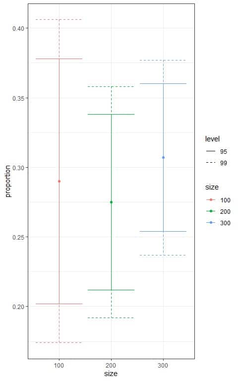
We see that:

• The confidence interval based on the 300 sample size is the narrowest interval.
• For each sample size, the 95% confidence interval (solid line) is tighter than the 99% confidence interval (dashed line).

6. Practice questions

1. The following plot shows the different 95% confidence intervals for the proportion of employed persons from a certain population based on different sample sizes.

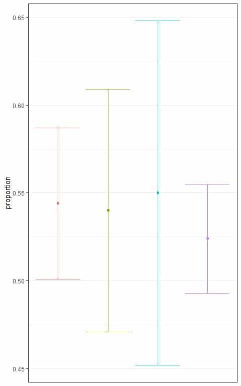
Which interval is based on the smallest sample size?

2. The following plot shows the different confidence intervals for the proportion of employed persons from a certain population based on different levels.

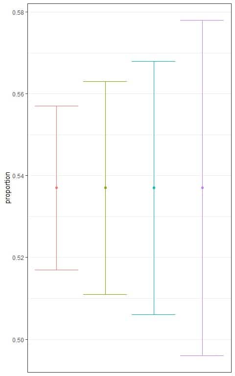
Which interval is based on the lowest level of confidence?

3. The following table shows some summary statistics of the annual income of some persons randomly sampled from a population.

Where n is the sample size and sd is the standard deviation.

What is the 95% and 99% confidence interval for the mean income of this population?

4. The following table shows some summary statistics of the infant mortality in deaths per 1000 births in Africa.

Where n is the sample size and sd is the standard deviation.

Assuming this is a random sample, what is the 95% confidence interval for the mean mortality rate in Africa?

5. A random sample of 1000 persons showed that 0.157 were divorced.

What are the 95% and 99% confidence intervals for the true divorced proportion in the population from which those persons were sampled?

7. Answer key

1. The blue interval because it is the widest interval.

The smallest sample size will lead to the largest standard error and the widest interval.

2. The red interval because it is the narrowest interval.

The lowest confidence will lead to the smallest number multiplied by the standard error and the narrowest interval.

3. Check for the needed sample conditions so that the sampling distribution of its mean is normal:

• The sample data must be independent. The data are randomly sampled from the population so they are independent.
• The sample should be of size ≥ 30 which is also true.

Use the sample standard deviation (s) to calculate the standard error SE.

SE=s/√n=35487.61/√84 = 3872.016.

95% confidence interval = ¯x±1.96XSE = 18768.45-1.96X3872.016 to 18768.45+1.96X3872.016 = 11179.3 to 26357.6.

99% confidence interval = ¯x±2.58XSE = 18768.45-2.58X3872.016 to 18768.45+2.58X3872.016 = 8778.649 to 28758.25.

4. Check for the needed sample conditions so that the sampling distribution of its mean is normal:

• The sample data must be independent. The data is a random sample so it is an independent sample.
• The sample should be of size ≥ 30 which is also true.

Use the sample standard deviation (s) to calculate the standard error SE.

SE=s/√n=54.943/√34 = 9.42.

95% confidence interval = ¯x±1.96XSE = 142.291-1.96X9.42 to 142.291+1.96X9.42 = 123.8278 to 160.7542.

We are 95% confident that the mean infant mortality rate (per 1000 births) in Africa is between 123.8278 and 160.7542.

5. Check for the needed sample conditions so that the sampling distribution of its proportion p ̂ is normal:

• The data must be independent.

The data are randomly sampled from a population so this condition is true.

• The np ̂≥10 and n(1-p ̂)≥10.

1000 X 0.157 = 157 and 1000 X (1-0.157) = 843. Both numbers are larger than 10 so this condition is true also.

Use the sample proportion p ̂ to calculate the standard error SE.

SE=√((p(1-p))/n)=√((0.157(1-0.157))/1000)=0.0115.

95% confidence interval = p ̂±1.96XSE = 0.157-1.96X0.0115 to 0.157+1.96X0.0115 = 0.134 to 0.18.

We are 95% confident that the true population proportion for divorced persons is between 0.134 and 0.18 or between 13.4% and 18%.

99% confidence interval = p ̂±2.58XSE = 0.157-2.58X0.0115 to 0.157+2.58X0.0115 = 0.127 to 0.187.

We are 99% confident that the true population proportion for divorced persons is between 0.127 and 0.187 or between 12.7% and 18.7%.

Previous Lesson | Main Page | Next Lesson