The Standard Deviation – Explanation & Examples

The definition of the standard deviation is:

“The standard deviation is a measure of the dispersion of a set of numerical values relative to their mean.”

In this topic, we will discuss the standard deviation from the following aspects:

• What is the standard deviation?
• How to calculate the standard deviation?
• Standard deviation formula.
• The role of the standard deviation.
• Practice questions.
• Answer key.

What is the standard deviation?

The standard deviation is a measure of the dispersion of a set of numerical values from their mean.

We calculate the standard deviation as the square root of the variance. The variance is the mean or average of the squared differences from the mean.

The variance has the squared unit of the numerical data due to squared differences in its calculation, so it is difficult to interpret.

Alternatively, the standard deviation has the same unit of the numerical data and is easier to interpret.

A large standard deviation indicates that your data numbers are far from the mean and far from each other. In contrast, a small standard deviation indicates that numbers in your data are more clustered around their mean.

A zero standard deviation indicates that all numbers within your data are identical.

– Example

Suppose you have two sets of 3 numbers (1,2,3) and (1,2,10). You see that the second set is more spread (more varied) than the first set.

You can see that from the following dot plot.

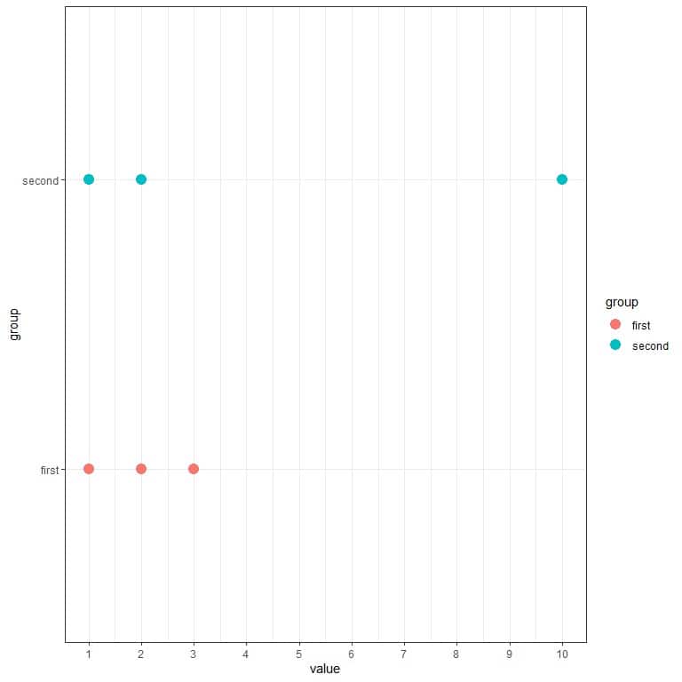
We see that the blue dots (second group) are more spread out than the red dots (first group).

Suppose we calculate the standard deviation for the first group. In that case, it is 1, while the standard deviation for the second group is 4.9. Therefore, the second group is more spread (more varied) than the first group.

How to calculate the standard deviation?

We will go through several examples, from simple to more complex ones.

– Example 1

What is the standard deviation of the numbers, 1,2,3?

1. Add up all of the numbers:

1+2+3 = 6.

2. Count the numbers of items in your data. In this data, there are 3 items.

3. Divide the number you found in step 1 by the number you found in step 2.

The mean = 6/3 = 2.

4. In a table, subtract the mean from each value of your data.

You have a table of 2 columns, one for the data values and the other column for subtracting the mean (2) from each value.

5. Add another column for the squared differences you found in Step 4.

6. Add up all of the squared differences you found in Step 5.

1+0+1 = 2.

7. Divide the number you get in step 6 by sample size-1 to get the variance. We have 3 numbers, so the sample size is 3.

The variance = 2/(3-1) = 1.

8. Take the square root of the variance to get the standard deviation.

The standard deviation = √1 = 1.

– Example 2

What is the standard deviation of the numbers, 1,2,10?

1. Add up all of the numbers:

1+2+10 = 13.

2. Count the numbers of items in your data. In this data, there are 3 items.

3. Divide the number you found in step 1 by the number you found in step 2.

The mean = 13/3 = 4.33.

4. In a table, subtract the mean from each value of your sample.

We have 2 columns, one for the data values and the other column for subtracting the mean (4.33) from each value.

5. Add another column for the squared differences you found in Step 4.

6. Add up all of the squared differences you found in Step 5.

11.09 + 5.43 + 32.15 = 48.67.

7. Divide the number you get in step 6 by sample size-1 to get the variance. We have 3 numbers, so the sample size is 3.

The variance = 48.67/(3-1) = 24.335.

8. Take the square root of the variance to get the standard deviation.

The standard deviation = √24.335 = 4.9.

– Example 3

The following is the weight (in kg) of 30 smoking individuals and 30 never-smoking individuals. What is the standard deviation of each sample?

For the smoker group:

1. Add up all of the weights:

Sum = 2108.3.

2. Count the numbers of items in your group. In this sample, there are 30 items or individuals.

3. Divide the number you found in step 1 by the number you found in step 2.

The sample mean = 2108.3/30 = 70.28 kg.

4. In a table, subtract the mean from each value of your sample.

5. Add another column for the squared differences you found in Step 4.

6. Add up all of the squared differences you found in Step 5.

Sum = 4013.57.

7. Divide the number you get in step 6 by sample size-1 to get the variance. We have 30 numbers, so the sample size is 30.

The variance = 4013.57/(30-1) = 138.399 kg^2.

8. Take the square root of the variance to get the standard deviation.

The standard deviation = √138.399 = 11.76 kg.

Note that the standard deviation has the same unit as the original data (kg).

For the never smoker group:

1. Add up all of the weights:

Sum = 2057.3.

2. Count the numbers of items in your group. In this sample, there are 30 items or individuals.

3. Divide the number you found in step 1 by the number you found in step 2.

The sample mean = 2057.3/30 = 68.58.

4. In a table, subtract the mean from each value of your sample.

5. Add another column for the squared differences you found in Step 4.

6. Add up all of the squared differences you found in Step 5.

Sum = 4819.3.

7. Divide the number you get in step 6 by sample size-1 to get the variance. We have 30 numbers, so the sample size is 30.

The variance = 4819.3/(30-1) = 166.18 kg^2.

8. Take the square root of the variance to get the standard deviation.

The standard deviation = √166.18 = 12.89 kg.

The never smoker weights are more variable than smoker weights. It is also evident from the following dot plot.

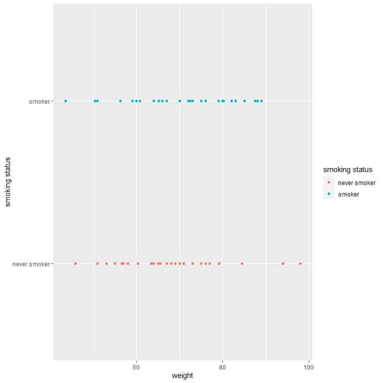
We see that the never smoker weights are more spread out than the smoker weights.

– Example 4

The following is a table for the weights of diamonds produced from 2 different machines. Which machine is better?

Note less variable weights means a more precise machine which is a good criterion. If the variability is high, the machine will produce many diamonds whose weights are out of the desired limits.

For machine_1:

1. Add up all of the numbers:

Sum = 9.

2. Count the numbers of items in your sample. In this sample, there are 35 items.

3. Divide the number you found in step 1 by the number you found in step 2.

The sample mean = 9/35 = 0.2571.

4. In a table, subtract the mean from each value of your sample.

5. Add another column for the squared differences you found in Step 4.

6. Add up all of the squared differences you found in Step 5.

Sum = 0.0479.

7. Divide the number you get in step 6 by sample size-1 to get the variance. Our sample size is 35.

The variance = 0.0479/(35-1) = 0.0014 grams^2.

8. Take the square root of the variance to get the standard deviation.

The standard deviation = √0.0014 = 0.037 grams.

For machine_2:

1. Add up all of the numbers:

Sum = 26.04.

2. Count the numbers of items in your sample. In this sample, there are 35 items.

3. Divide the number you found in step 1 by the number you found in step 2.

The sample mean = 26.04/35 = 0.744.

4. In a table, subtract the mean from each value of your sample.

5. Add another column for the squared differences you found in Step 4.

6. Add up all of the squared differences you found in Step 5.

Sum = 0.255.

7. Divide the number you get in step 6 by sample size-1 to get the variance. Our sample size is 35.

The variance = 0.255/(35-1) = 0.0075 grams^2.

8. Take the square root of the variance to get the standard deviation.

The standard deviation = √0.0075 = 0.087 grams.

machine_2 weights are more variable than machine_1 weights. We can see that if we plot the data as a dot plot.

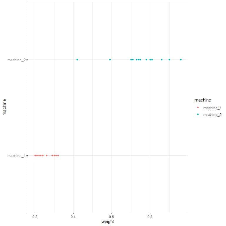
We see that machine_1 weights occupy a smaller numerical range than machine_2 weights.

Standard deviation formula

The standard deviation formula is:

s=√((∑_(i=1)^n▒( x_i-¯x )^2)/(n-1))

Where s is the standard deviation.

¯x is the sample mean.

n is the sample size.

The term:

∑_(i=1)^n▒( x_i-¯x )^2

means sum the squared difference between every element of our sample (from x_1 to x_n) and the sample mean ¯x.

Our sample element is denoted as x with a subscript to indicate its position in our sample.

In the example of diamonds’ weights for machine_1, we have 35 weights. The first weight (0.23) is denoted as x_1, the second weight (0.21) is denoted as x_2, the third weight (0.23) is denoted as x_3And the last weight (0.23) is denoted as x_35 or x_n because n = 35 in this case.

We used this formula in the above examples, where we summed the squared difference between every element of our data and the sample mean, then divided by the sample size-1 or n-1 to get the variance. Finally, we took the square root of the variance to get the standard deviation.

We divide by n-1 when calculating the variance or the standard deviation (and not by n as any average) to make the sample standard deviation a good estimator of the true population standard deviation.

However, if you have population data, you will divide by N (where N is the population size) to get the standard deviation.

Example

We have a population of more than 20,000 individuals. From the census data, the population standard deviation for the age was 17.29 years.

We take a random sample of 50 individuals from this data. The sum of squared differences from the mean was 12112.08.

If we divide by 50 (sample size), the variance will be 242.24, and the standard deviation will be 15.56.

If we divide by 49 (sample size-1), the variance will be 247.19, and the standard deviation will be 15.72.

Dividing by n-1 will make the variance and standard deviation a bit larger and prevent them from underestimating the true population variance or standard deviation.

The role of the standard deviation

The standard deviation is a summary statistic used to give information about your data or population’s spread.

In the above example of two machines, although we have only a sample of 35 diamonds from each machine, we can conclude that (with some level of certainty) that machine_2 is more variable (and so worse) than machine_1.

When some machines produce a certain product with a high standard deviation for certain criteria (like weight for diamonds), these machines need adjustment.

Standard deviation is also important in an investment where standard deviation (as a measure of spread or variability) can be used to measure risk.

Stocks prices with greater standard deviations are riskier to invest in.

Disadvantages of standard deviation as a measure of spread:

It is affected by outliers. These are the numbers that are far from the mean.

Practice questions

1. The following table is the daily closing prices (in USD) of 3 stocks from the information technology sector, Apple (AAPL), Microsoft (MSFT), and Adobe (ADBE), for some days in 2006. Which stock has the least standard deviation for the closing prices?

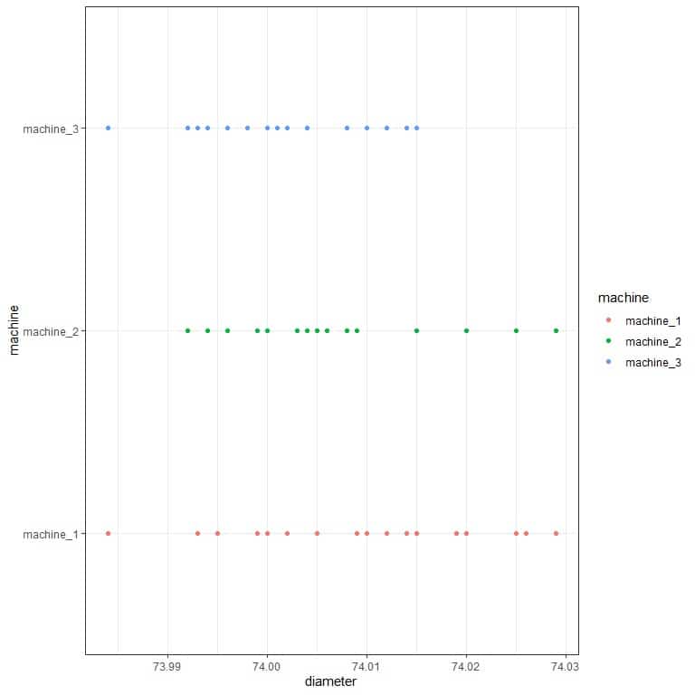
2. The following is a table of the inside diameter (in mm) for piston rings produced from 3 different machines. Which machine is more precise in its production?

Note more precise means less variable.

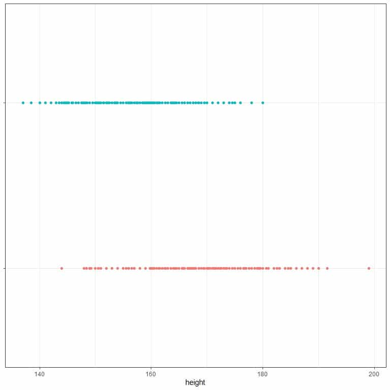
3. The following is the standard deviation for heights of females and males from a certain population. Also, dot plots for the height values. Which dots are males, and which are females?

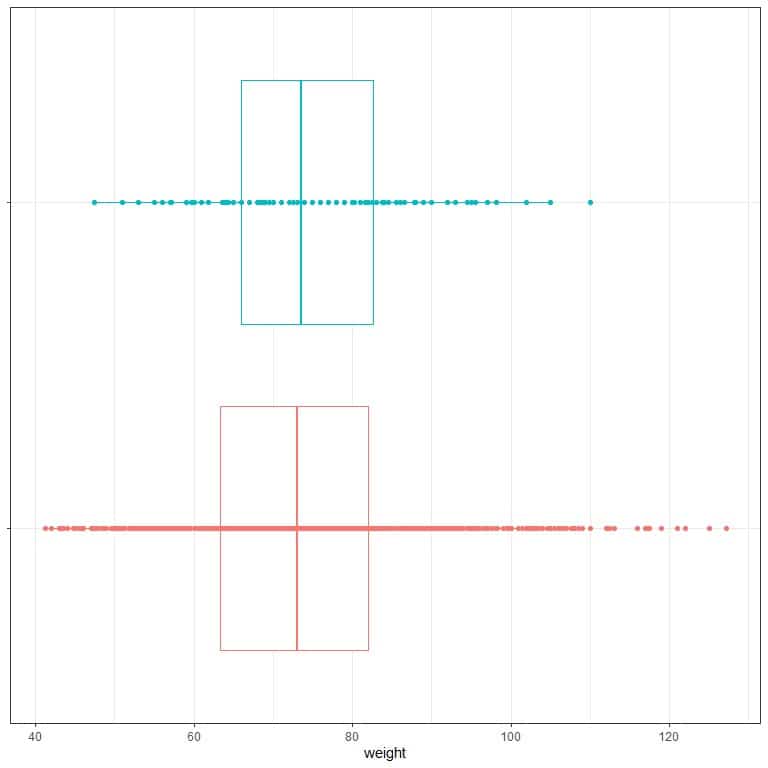
4. The following is the standard deviation for weights of individuals who had a cardiovascular event (cv) and other individuals who did not have this event from a certain population. Also, box plots and dot plots for the weight values. Which dots are individuals with cardiovascular events?

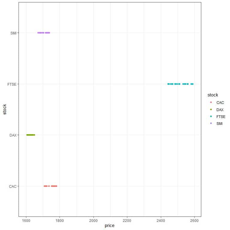
5. The following are the daily closing prices of major European stock indices: Germany DAX (Ibis), Switzerland SMI, France CAC, and UK FTSE for some days in 1991. Which stock has the most standard deviation?

Answer key

1. We will calculate the standard deviation for each stock then compare them.

• Add up all of the numbers:

Sum for Apple = 247.6557.

Sum for Microsoft = 680.06.

Sum for Adobe = 882.17.

• Count the numbers of items in your sample. In this sample of each stock, there are 30 items.
• Divide the number you found in step 1 by the number you found in step 2.

The mean for Apple = 247.6557/30 = 8.255.

The mean for Microsoft = 680.06/30 = 22.67.

The mean for Apple = 882.17/30 = 29.41.

• Subtract the mean of each stock from each value of this stock and square the difference.

• Add up all of the squared differences you found in Step 4 for each stock.

Sum of squared differences for Apple = 2.98.

Sum of squared differences for Microsoft = 10.41.

Sum of squared differences for Adobe = 19.51.

• Divide the number you get in step 5 by sample size-1 to get the variance. We have 30 numbers, so the sample size is 30.

The variance of Apple closing price = 2.98/(30-1) = 0.10 USD^2.

The variance of Microsoft closing price = 10.41/(30-1) = 0.36 USD^2.

The variance of Adobe closing price = 19.51/(30-1) = 0.67 USD^2.

• Take the square root of the variance to get the standard deviation.

The standard deviation of Apple = √0.10 = 0.32 USD.

The standard deviation of Microsoft = √0.36 = 0.60 USD.

The standard deviation of Adobe = √0.67 = 0.82 USD.

The Apple stock closing price has the least standard deviation. We can see that if we plot the data as a dot plot.

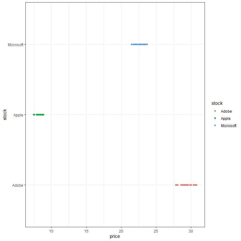We see that the Apple prices are less scattered than Adobe or Microsoft prices.

2. After doing similar calculations of question 1, we get the following table for each machine’s standard deviation.

Machine_3 has the least standard deviation, and so it is more precise than the other 2 machines. We can see that if we plot the data as a dot plot.

3. Red dots are males (more dispersed), and blue dots are females.

4. Individuals with cv events have a lower standard deviation, so they are the blue dots.

5. After doing similar calculations of question 1, we get the following table for each stock’s standard deviation.

The FTSE has the most standard deviation, and so it is riskier than the other 3 stocks. We can see that if we plot the data as a dot plot.

Previous Lesson | Main Page | Next Lesson