Vector Fields – Definition, Graphing Technique, and Example
Vector fields allow us to exhibit relationships between objects that expand over a wide region of the plane (or even space). In Physics, for example, we use vector fields to describe the object’s magnetic or electric fields. These are also essential when studying large-scale occurrences such as the varying motions of water in a river or the gravitational field between astronomical objects, so we must understand how vector fields work.
Have you seen diagrams filled with arrows (or vectors) in a plane or space? We call these diagrams a vector field. A vector field within a domain of either a plane or a space represents a vector-valued function. For each point in the plane (or space), the vector field assigns a vector that is associated with it.
In this article, we’ll learn how the algebraic representations of vector fields. We’ll also show you how to construct vector fields and learn how to represent vector functions as vector fields.
What Is a Vector Field?
A vector field represents the region in a plane or space that contains a group of vectors that satisfy a function, $\textbf{F}(x, y)$ in $ \mathbb{R}^2$ or $\textbf{F}(x, y, z)$ in $\mathbb{R}^3$. The diagram below shows an example of a vector field defined by the function, $\textbf{F}(x, y) = x \textbf{i} + y\textbf{j}$.
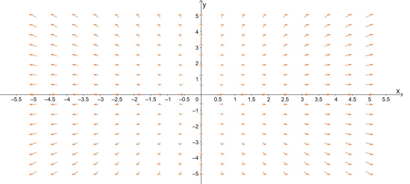
The diagram below shows an example of a vector field defined by the function, $\textbf{F}(x, y) = x \textbf{i} + y\textbf{j}$. This is how vector fields would appear when working with two-variables functions in $\mathbb{R}^2$. In general, we can write vector fields in $\mathbb{R}^2$ using the two forms shown below:
\begin{aligned}\textbf{F}(x, y) &=
Keep in mind that vector fields are continuous when the components of the function are continuous as well. Vector fields such as the radial and rotational fields are represented in the $xy$-plane with graphs that look similar to the diagram shown above. Before we learn how to draw more vector fields, let us first show you how to find a vector associated with a given point.
\begin{aligned}\textbf{F}(x, y) &= (x^2 – 3xy + 1)\textbf{i} – \sin y \textbf{j}\\ (x, y) &= (4, 0)\end{aligned}
Simply substitute $(x, y) = (4, 0)$ into the vector function to determine a vector associated with $(4, 0)$.
\begin{aligned}\textbf{F}(4, 0) &= (4^2 – 3\cdot 4\cdot 0 + 1)\textbf{i} – \sin 0 \textbf{j}\\ &= 5\textbf{i} – \textbf{j}\\&= <5, 1>\end{aligned}
This step is crucial in the later section when we start learning how to construct vector fields given a vector function.
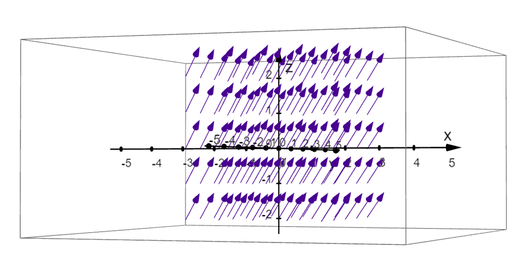
We can also represent three-variable functions as a vector field in space or $mathbb{R}^3$. The graph above shows the visual representation of the function, $\textbf{F}(x,y, z) = 1\textbf{i} – 1\textbf{j} + 1 \textbf{k}$. As with planar vector fields, we can write the equation of the vector field in $\mathbb{R}^3$ as shown below.
\begin{aligned}\textbf{F}(x, y, z) &=
Apply a similar process to find a vector in space associated with $\textbf{F}(x, y, z)$ that passes through the point, $(x_o, y_o, z_o)$. We use vector fields in $\mathbb{R}^3$ when representing large regions such as gravitational fields. In the next section, we’ll learn how to represent different vector functions by constructing their graphs in a plane or in space.
How to Graph Vector Fields?
We can graph the vector field using the components of the vector function or the given unit vectors of the function. Did you know that the actual graph of a vector field has at least four dimensions? That’s why we simplify its representation by constructing a vector field in $\mathbb{R}^2$.
Here’s a breakdown of the steps to remember when sketching the vector field in a 2D-coordinate system:
- Construct vectors that are associated with the function and some given points (be strategic when selecting these points.
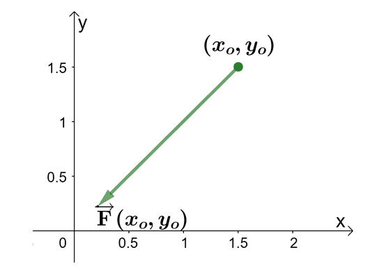
- From $(x_o, y_o)$, use the components of the vector, $\textbf{F}(x _o, y_o)$ to construc the vector.
- Use the rest of the table of values to graph the rest of the vectors.
- Try to scale the vectors so that the arrows won’t make the vector field appear “messy”. Reduce the vector lengths by less than $50\%$ or depending on what makes the graph neater like the vector field shown below.
Another way for us to scale vectors in these diagrams is by normalize the vectors to shorten lengths of the vectors.
To better understand how the process works, let’s go ahead and sketch the vector field, $\textbf{F}(x, y) = 2x \textbf{i} + 2y \textbf{j}$. We begin by finding vectors throughout the four quadrants of the two-dimensional coordinate system. Evaluate each assigned point to find the components of the vectors.
\begin{aligned}(x, y)\end{aligned} | \begin{aligned}\textbf{F}(x, y)\end{aligned} | \begin{aligned}(x, y)\end{aligned} | \begin{aligned}\textbf{F}(x, y)\end{aligned} |
\begin{aligned}\left(\dfrac{1}{2}, 0 \right)\end{aligned} | \begin{aligned}\left<1, 0\right>\end{aligned} | \begin{aligned}\left(-\dfrac{1}{2}, \dfrac{1}{2} \right)\end{aligned} | \begin{aligned}\left< -1,1\right>\end{aligned} |
\begin{aligned}\left(0, \dfrac{1}{2} \right)\end{aligned} | \begin{aligned}\left<0,1\right>\end{aligned} | \begin{aligned}\left(-\dfrac{1}{2}, -\dfrac{1}{2} \right)\end{aligned} | \begin{aligned}\left< -1,-1\right>\end{aligned} |
\begin{aligned}\left(-\dfrac{1}{2}, 0 \right)\end{aligned} | \begin{aligned}\left<-1,0\right>\end{aligned} | \begin{aligned}\left(1, 0 \right)\end{aligned} | \begin{aligned}\left<2, 0\right>\end{aligned} |
\begin{aligned}\left(0, -\dfrac{1}{2}\right)\end{aligned} | \begin{aligned}\left<0,-1\right>\end{aligned} | \begin{aligned}\left(0, 1 \right)\end{aligned} | \begin{aligned}\left<0,2\right>\end{aligned} |
\begin{aligned}\left(\dfrac{1}{2}, \dfrac{1}{2} \right)\end{aligned} | \begin{aligned}\left<1,1\right>\end{aligned} | \begin{aligned}\left(-1, 0 \right)\end{aligned} | \begin{aligned}\left<-2,0\right>\end{aligned} |
\begin{aligned}\left(\dfrac{1}{2}, -\dfrac{1}{2} \right)\end{aligned} | \begin{aligned}\left<1,-1\right>\end{aligned} | \begin{aligned}\left(0, -1\right)\end{aligned} | \begin{aligned}\left<0,-2\right>\end{aligned} |
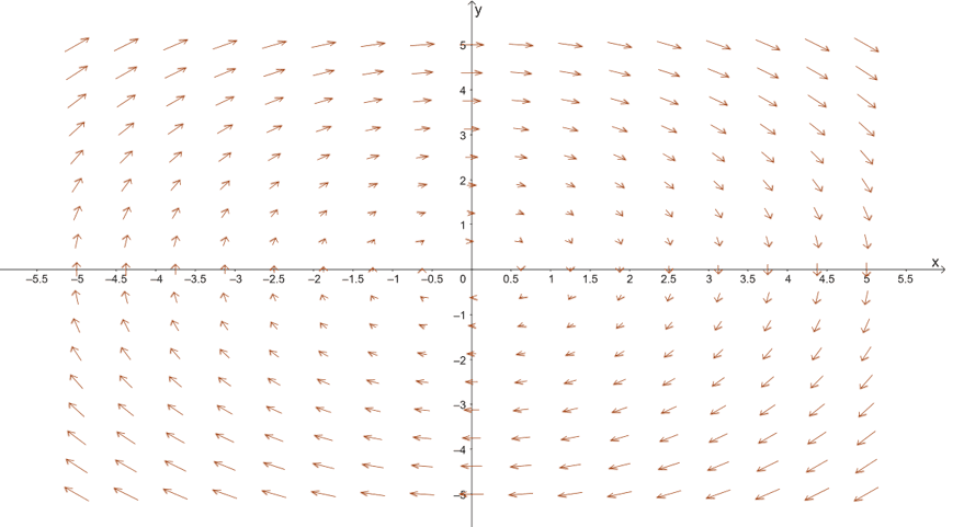
Use these vectors and sketch some of them on the $xy$-plane to give you an idea of how the vector field’s shape would look like.
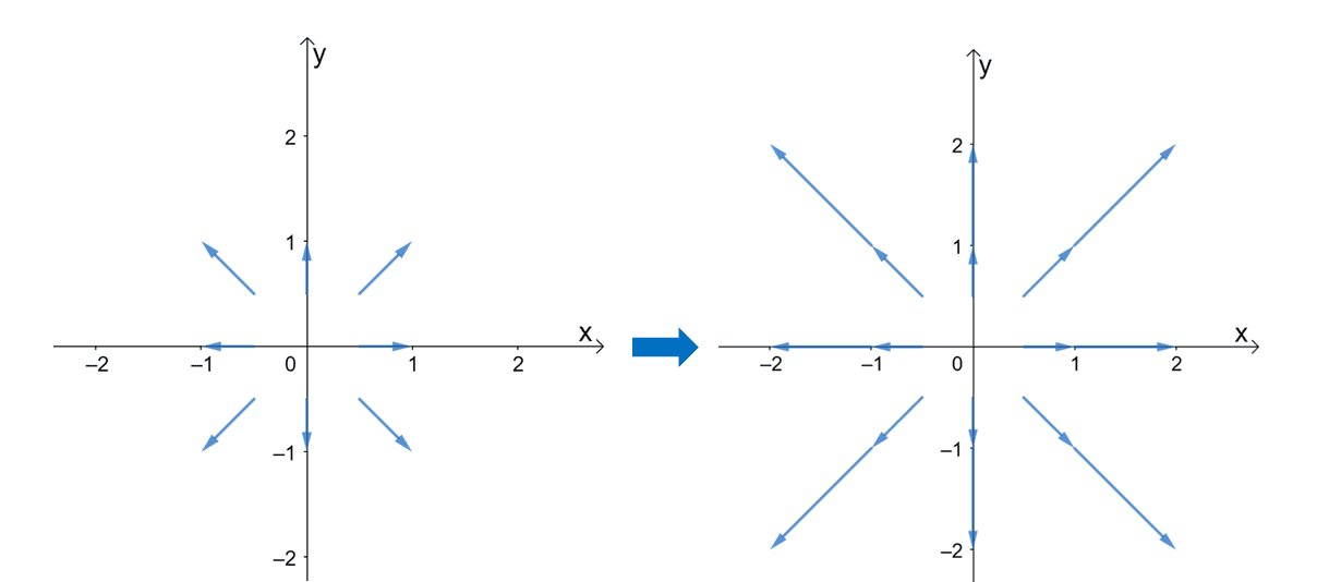
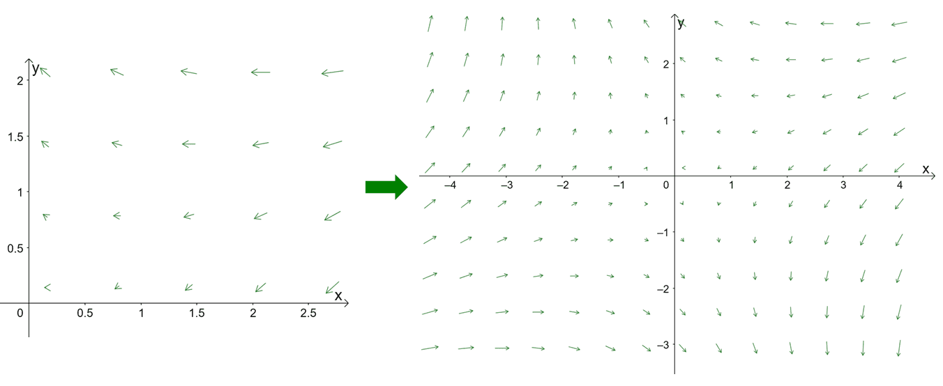
Plotting more vectors will give us a better visualization of how the vector field would look like. Once you’ve constructed more vectors and scaling the length of the vector so they look more uniform, then you’ll have the vector field shown below.
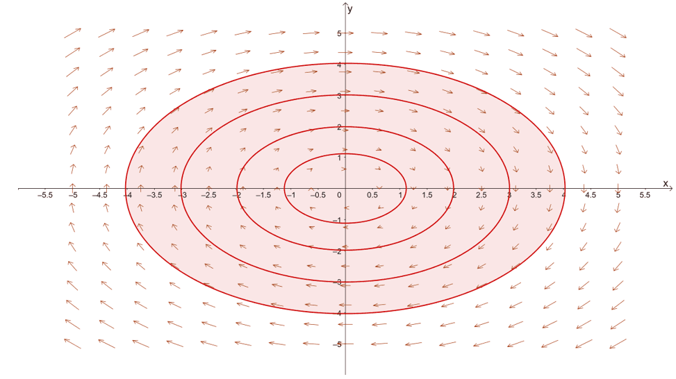
The right graph represents the vector field for $\textbf{F}(x, y) = <2x, 2y> = 2 \textbf{i} + 2 \textbf{j}$. We’ve included a second graph on the left – how the vector field would look like with three concentric circles graphed over them. We graphed the circles to highlight an important property of the vector field: the vectors are perpendicular to these circles. Hence, we call these vector fields the radial vector fields.
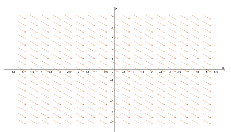
Graphing vector fields in $\mathbb{R}3$ requires us to use computing and graphing systems. Most of the time, it is impossible for us to sketch vector fields by hand alone. For simpler vector-valued functions such as $\textbf{F}(x, y, z) = <2, ,2, z>$, we use the constants to determine which of the components will remain constant. For this example, the $x$ and $y$ components are constant, so we can visualize how the vector field looks like on the $xy$-plane.
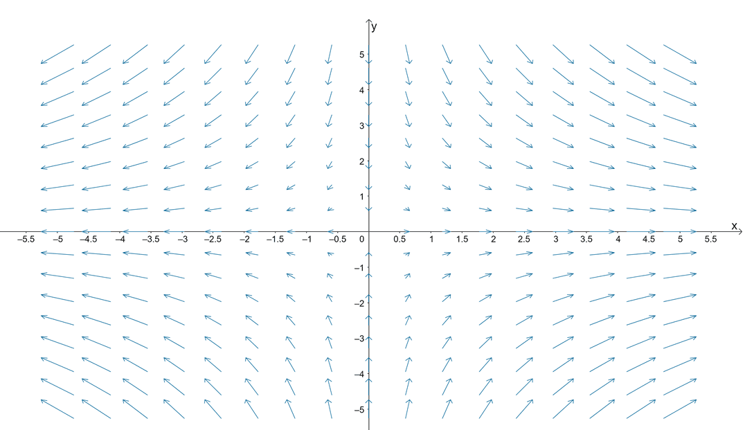
This diagram represents the vector field, $\textbf{F}(x, y) = <2, 2>$. This means that the direction of the vectors along the plane when $z= 0$ would look like this. This helps us predict how the rest of the vectors along different values of $z$ would look like – shifting the vectors above or below. Of course, computing or graphing systems will still be the way to go if you want a more accurate visualization of $\textbf{F}(x,y, z) = <2, 2, z>$.
Here’s the diagram of the vector field representing $\textbf{F}(x, y) = <2, 2>$ in $\mathbb {R}^3$. We used GeoGebra to graph this 3D vector field, but you can definitely use other graphing systems!
Now that we’ve shown you the process of graphing vector fields in $\mathbb{R}^2$ and $\mathbb{R}^3$, it’s time for you to try graphing them yourself! When you’re ready, head over to the next section and work on more problems involving vector fields.
Example 1
Given that $\textbf{G}(x, y) = 4x^2y \textbf{i} – (2x + y)\textbf{j}$ is a vector field in $\mathbb{R}^2$. Determine the vector that is associated with $(-1, 4)$.
Solution
To find the vector associated with a given point and vector field, we simply evaluate the vector-valued function at the point: let’s evaluate $\textbf{G}(-1, 4)$.
\begin{aligned}\textbf{G}(x, y) &= 4x^2y \textbf{i} – (2x + y)\textbf{j}\\\textbf{G}(-1, 4) &= 4(-1)^2(4) \textbf{i} – [2(-1) + (4)]\textbf{j}\\&= -16 \textbf{i} – 2\textbf{j}\end{aligned}
This means that the vector associated $\textbf{G}(x, y)$ and the point, $(-1, 4)$, is equal to $\textbf{G}(-1, 4) = -16 \textbf{i} – 2\textbf{j} = <-16, -2>$.
Example 2
Prove that $\textbf{F}(x, y) = \left<\dfrac{x}{\sqrt{x^2 + y^2}}, \dfrac{y}{\sqrt{x^2 + y^2}}\right>$ , is a unit vector field.
Solution
When given a vector field, we can show that it is a unit vector field by checking if its magnitude is equal to $1$. Recall that we can calculate the magnitude of the vector function by adding the squares of the components and taking the square root of the result.
\begin{aligned}\end{aligned}\begin{aligned}\left| \left<\dfrac{x}{\sqrt{x^2 + y^2}}, \dfrac{y}{\sqrt{x^2 + y^2}}\right>\right| &= \sqrt{\dfrac{x^2}{x^2 + y^2} + \dfrac{y^2}{x^2 + y^2}}\\&= \sqrt{\dfrac{x^2 + y^2}{x^2 + y^2}} \\&= \sqrt{1}\\ &=1\end{aligned}
Since the resulting magnitude is equal to $1$, we can confirm that the vector field is a unit vector field. Unit vector fields are helpful in constructing our vector field diagrams because they help us normalize the vectors so that we’re creating diagrams with uniform-looking vectors.
Example 3
Graph the vector field, $\textbf{F}(x, y) = -y \textbf{i} + x \textbf{j}$.
Solution
When sketching vector fields, our first goal is to set up a table of values containing vectors evaluated from selected points. Here’s a summary of the vectors associated with the following points:
\begin{aligned}(x, y)\end{aligned} | \begin{aligned}\textbf{F}(x, y)\end{aligned} | \begin{aligned}(x, y)\end{aligned} | \begin{aligned}\textbf{F}(x, y)\end{aligned} |
\begin{aligned}(1, 0) \end{aligned} | \begin{aligned} <0, 1> \end{aligned} | \begin{aligned}(1, -1) \end{aligned} | \begin{aligned} <1, 1>\end{aligned} |
\begin{aligned}(0, 1) \end{aligned} | \begin{aligned} <-1, 0> \end{aligned} | \begin{aligned}(-1, -1) \end{aligned} | \begin{aligned} <1, -1>\end{aligned} |
\begin{aligned}(-1, 0) \end{aligned} | \begin{aligned} <0, -1>\end{aligned} | \begin{aligned}(2, 0) \end{aligned} | \begin{aligned} <0, 2>\end{aligned} |
\begin{aligned}(0, -1) \end{aligned} | \begin{aligned} <1, 0>\end{aligned} | \begin{aligned}(0, 2) \end{aligned} | \begin{aligned} <-2, 0>\end{aligned} |
\begin{aligned}(1, 1) \end{aligned} | \begin{aligned} <-1, 1>\end{aligned} | \begin{aligned}(-2, 0) \end{aligned} | \begin{aligned} <0, -2>\end{aligned} |
\begin{aligned}(-1, 1) \end{aligned} | \begin{aligned} <-1, -1> \end{aligned} | \begin{aligned}(0, -2) \end{aligned} | \begin{aligned} <2, 0>\end{aligned} |
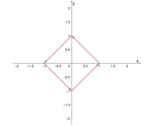
Now that we have our initial vectors, it’s time for us to graph these vectors on the $xy$-plane. For example, if we have $(1, 0)$ as the point, we graph the vector with $(1, 0)$ as its initial point and $(0, 1)$ as the endpoint. Do the same for the first four vectors and you should have the graph shown below.
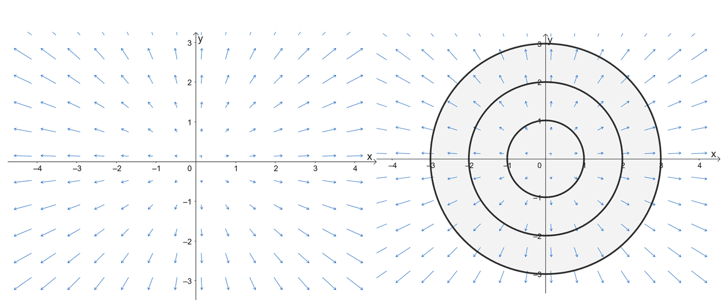
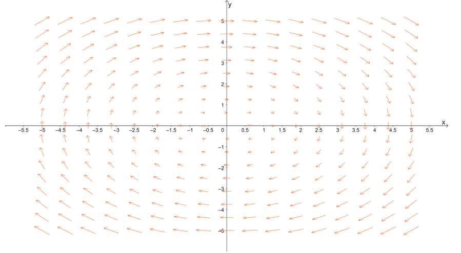
Continue sketching more vectors just to give us an idea of how the vector field’s vectors would behave. After graphing more vectors, you’ll see that the vector field contains vectors that rotate in a counterclockwise direction.
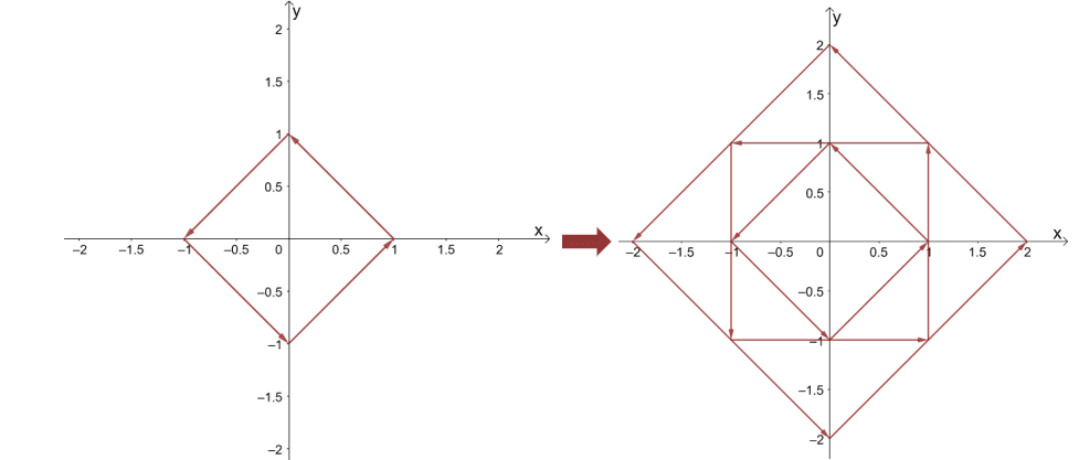
If we continue sketching more vectors, we’ll end up with the vector field shown below. As we have expected, the vectors look like they’re rotating around the center in a counterclockwise direction.
We call this type of vector field the rotational vector field – vector fields with vectors rotating around in a clockwise or counterclockwise direction. Unlike radial fields, the vectors, %%EDITORCONTENT%%lt;x_o, y_o>$, contained within the vector field are all tangent to the circle with a radius of $\sqrt{x_o^2 + y_o^2}$. The diagram below highlights this special property of rotational vector fields.
Example 4
Graph the vector field, $\textbf{G}(x, y, z) = <1, z, -1>$.
Solution
As we have mentioned earlier, it’s best to sketch the final graph of a vector field in $\mathbb{R}^3$ using graphing software. Of course, that doesn’t mean we won’t be able to predict how the graph of $\textbf{G}(x, y, z) = <1, z, -1>$ would look like.
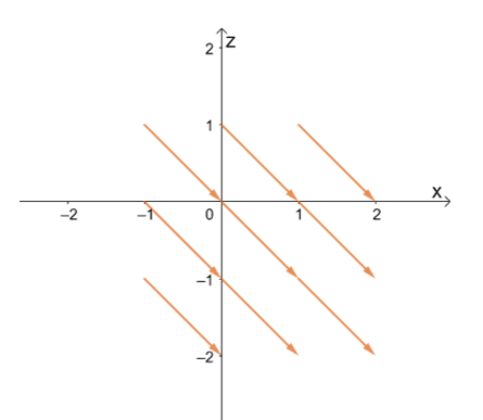
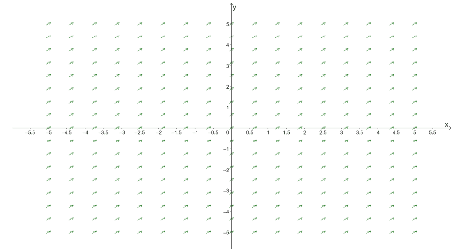
To start sketching the vectors, assign points for $(x, z)$ and from the point, move $1$ unit to the right then move $1$ unit downward. This position will be the endpoint of the vector. Try graphing the nine vectors shown above using this process. Once you have the hang of it, continue graphing more vectors and it should lead you to the vector field in $xz$-plane as shown below.
This gives you an idea of the direction of the vectors once we generate the graph of the vector field in $\mathbb{R}^3$. Since $y$ is dependent on the value of $z$, we use this fact to predict how the planes would behave in space.
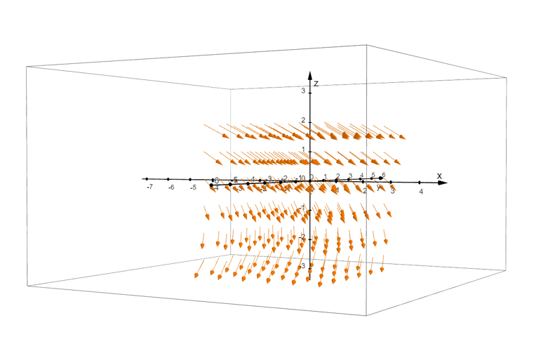
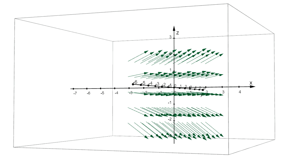
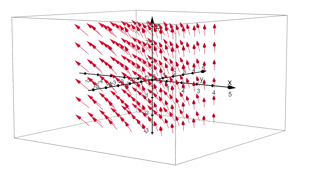
The graph above shows the generated vector field, $\textbf{G}(x, y, z) = <1, z, -1>$, in space. As we have predicted, the arrows are facing downwards and their positions only vary with respect to $z$. Use a computing system and try to generate this vector field in a three-dimensional coordinate system and see if it looks similar to the one we presented for you!
Practice Questions
1. Given that $\textbf{F}(x, y) = -3xy^3 \textbf{i} – (4x – y)\textbf{j}$ is a vector field in $\mathbb{R}^2$. Determine the vector that is associated with $(1, 1)$.
2. Given that $\textbf{G}(x, y, z) = 2xz^2 \textbf{i} + 3xz\textbf{j} + xy \textbf{k}$ is a vector field in $\mathbb{R}^3$. Determine the vector that is associated with $(-1, 0, 2)$.
3. Prove that $\textbf{F}(x, y) = \left<\sqrt{x} , \sqrt{1 – x}\right>$ , is a unit vector field.
4. Graph the vector field, $\textbf{F}(x, y) = 2y \textbf{i} – 2x \textbf{j}$.
5. Graph the vector field, $\textbf{F}(x, y) = \dfrac{x}{4} \textbf{i} – \dfrac{y}{4} \textbf{j}$.
6. Graph the vector field, $\textbf{G}(x, y, z) =
Answer Key
1.$\textbf{F}(1, 1) = -3\textbf{i} – 3\textbf{j} = <-3, -3>$
2.$\textbf{G}(-1, 0, 2) = -8\textbf{i} – 6\textbf{j} = <-8, -6>$
3.
$\begin{aligned}\end{aligned}\begin{aligned}\left| \left<\sqrt{x}, \sqrt{1- x}\right>\right| &= \sqrt{(\sqrt{x})^2 + (\sqrt{ 1- x})^2 }\\&= \sqrt{1} \\&=1\end{aligned}$
4.
5.
6.
Images/mathematical drawings are created with GeoGebra.