Z-Score – Explanation & Examples

The definition of the Z-score is:

“The Z-score is the number of standard deviations by which an observed value is above or below the mean value.”

In this topic, we will discuss the Z-score from the following aspects:

1. What is Z-score?
2. Z-score formula.
3. Z-score properties.
4. How to calculate Z-score?
5. The role of Z-score.
6. Practice questions.
7. Answer key.

1. What is Z-score?

The Z-score (standard score) is the number of standard deviations by which an observed value is above or below the mean value.

The Z-score is positive if the value lies above (greater than) the mean, and negative if the value lies below (smaller than) the mean.

For example, if the Z-score for an individual height is +1. This means that his height is 1 standard deviation above the mean height of his population.

On the other hand, if the Z-score for the same individual weight is -1. This means that his weight is 1 standard deviation below the mean weight of his population.

The Z-score can be 0 if the observed value exactly equals the mean.

The Z-score is used when the distribution of data, plotted as a histogram, nearly follows a normal distribution curve (a bell-shaped symmetrical curve centered around the mean).

– Example 1

The following are the histograms of heights, physical activity, and mental component summary from a certain population.

The mean value was plotted as a red dashed vertical line for each data.

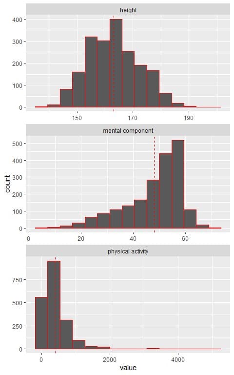
We see that:

• The histogram of height nearly follows a normal distribution curve (a bell-shaped symmetrical curve centered around the mean).
• The histogram of the mental component shows a left-skewed distribution (low frequent small values).
• The histogram of physical activity shows a right-skewed distribution (low frequent large values).

The Z-score can be applied to an individual’s height but cannot be applied to an individual’s mental component or physical activity.

However, there are different normal distributions with different means and standard deviations.

– Example 2

The following are the histograms of heights and weights from a certain population.

The mean value was plotted as a red dashed vertical line for each data.

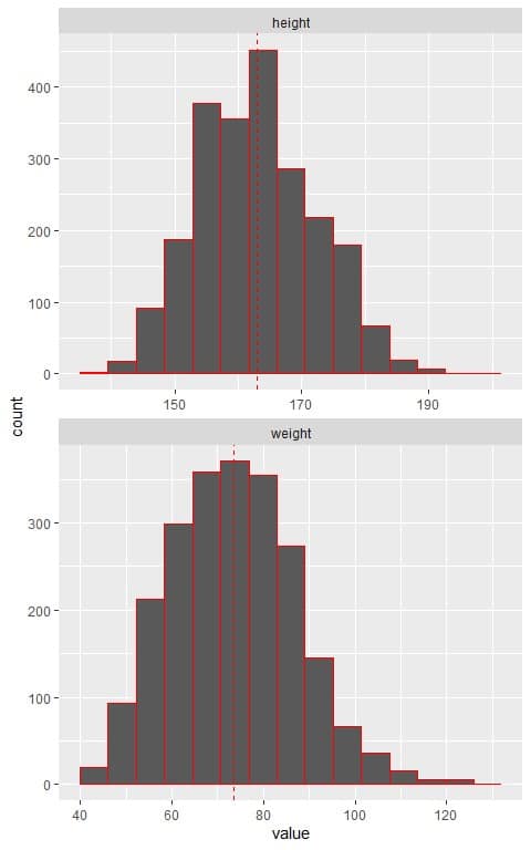
We see that:

• The histogram of heights and weights nearly follows a normal distribution curve (a bell-shaped curve).
• However, the mean value for heights was at about 165 (cm), while the mean value for weights was about 75 (kg).

– Example 3

In the above example, the mean height was 163 cm and standard deviation = 9.22 cm, while the mean weight was 73.4 kg and the standard deviation = 13.7 kg.

Assuming that heights and weights from this population follow the normal distribution, we can plot the normal distribution curves for heights and weights as follows:

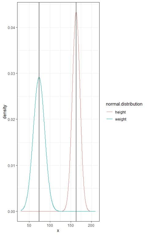
We see that:

• Each normal distribution curve is bell-shaped, peaked, and symmetric about its mean.
• When the standard deviation increases as for weights, the curve flattens away.

The Z-score converts all different normal distributions to a standard normal distribution with mean = 0 and standard deviation = 1.

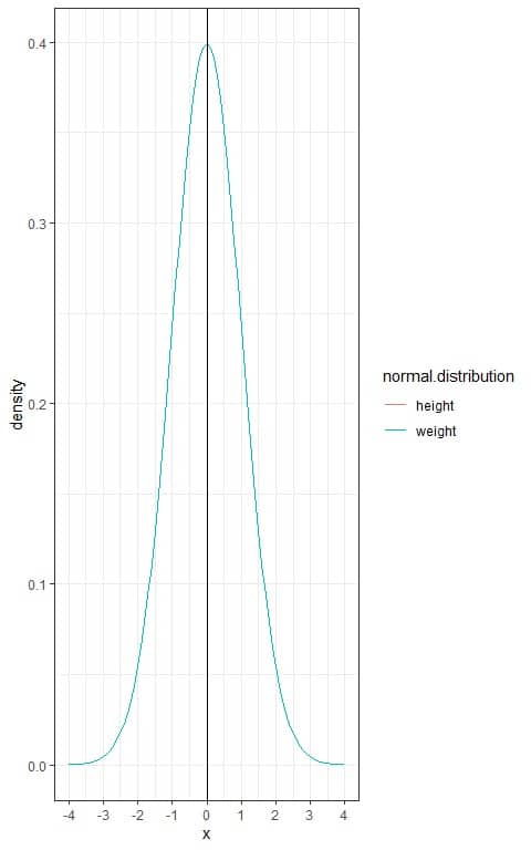
We see that:

• The two curves are superimposed over each other.
• Both heights and weights are now with a mean = 0 and standard deviation = 1.
• The Z-score allows the comparison of values (as heights and weights) from different normal distributions by standardizing their distribution.

2. Z-score formula

The Z-score formula is:

Z=(x-μ)/σ

where:

x is the data point.

μ is the population mean.

σ is the population standard deviation.

When the population mean and the population standard deviation are unknown, the Z-score can be calculated using the sample mean (¯x) and sample standard deviation (s) as estimates of the population values.

3. Z-score properties

As the Z-score forms a standard normal distribution with mean = 0 and standard deviation = 1, so it follows the properties of the normal distribution as the 68-95-99.7% rule.

The following is the normal distribution curve for any Z-score:

The important properties of normal distribution, that the Z-score follows, are:

• 68% of the data are within 1 standard deviation from the mean.

This means that 68% of the population has Z-score between +1 and -1. In other words, the probability of data from this population to lie between +1 and -1 Z-score is 68%.

As the normal distribution is symmetric around its mean, so 34% (68%/2) of this population have Z-score between 0 (mean) and +1 and 34% of this population have Z-score between -1 and 0.

If we shade the area within 1 standard deviation from the mean or between -1 and +1.

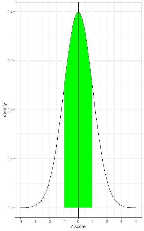
Without doing integration for this green AUC, the green shaded area represents 68 % of the total area, or the data within -1 and +1 Z-score represents 68% of the total data.

• 95% of the data are within 2 standard deviations from the mean.

This means that 95% of the population has Z-score between +2 and -2. In other words, the probability of data from this population to lie between +2 and -2 Z-score is 95%.

As the normal distribution is symmetric around its mean, so 47.5% (95%/2) of this population have Z-score between 0 (mean) and +2 and 47.5% of this population have Z-score between -2 and 0.

If we shade the area within 2 standard deviations from the mean or between -2 and +2.

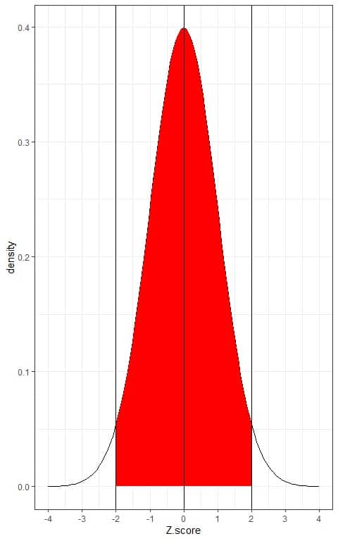
Without doing integration for this red AUC, the red shaded area represents 95% of the total area, or the data within -2 and +2 Z-score represents 95% of the total data.

• 99.7% of the data are within 3 standard deviations from the mean.

This means that 99.7% of the population has Z-score between +3 and -3. In other words, the probability of data from this population to lie between +3 and -3 Z-score is 99.7%.

As the normal distribution is symmetric around its mean, so 49.85% (99.7%/2) of this population have Z-score between 0 (mean) and +3 and 49.85% of this population have Z-score between -3 and 0.

If we shade the area within 3 standard deviations from the mean or between -3 and +3.

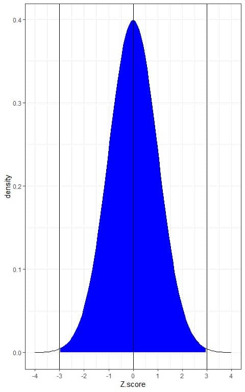
Without doing integration for this blue AUC, the blue shaded area represents 99.7% of the total area, or the data within -3 and +3 Z-score represents 99.7% of the total data.

• The proportion (probability) of data that are larger than the mean = probability of data that are less than the mean = 0.50 or 50%.

This means that 50% of the population has Z-score more than 0 and the other half has Z-score smaller than 0.

In other words, the probability of data from this population to be more than 0 Z-score = the probability of data from this population to be less than 0 Z-score = 50%.

This is plotted as follows:

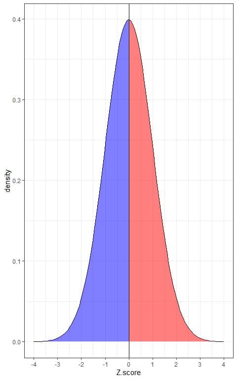
The blue shaded area = probability that the data has a Z-score less than 0 = 0.5 or 50%.

The red shaded area = probability that the data has a Z-score more than 0 = 0.5 or 50%.

• The probability of data that are larger than 1 standard deviation from the mean = the probability of data that are smaller than 1 standard deviation from the mean= 0.16 or 16%.

This means that 16% of the population has Z-score more than 1 and another 16% of the population has Z-score smaller than -1.

In other words, the probability of data from this population to have more than 1 Z-score = the probability of data from this population to have less than -1 Z-score = 16%.

This is plotted as follows:

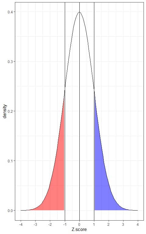
The blue shaded area = probability that the data has a Z-score more than 1 = 0.16 or 16%.

The red shaded area = probability that the data has a Z-score less than -1 = 0.16 or 16%.

• The probability of data that are larger than 2 standard deviations from the mean= the probability of data that are smaller than 2 standard deviations from the mean= 0.025 or 2.5%.

This means that 2.5% of the population has Z-score more than 2 and another 2.5% of the population has Z-score smaller than -2.

In other words, the probability of data from this population to have more than 2 Z-score = the probability of data from this population to have less than -2 Z-score = 2.5%.

This is plotted as follows:

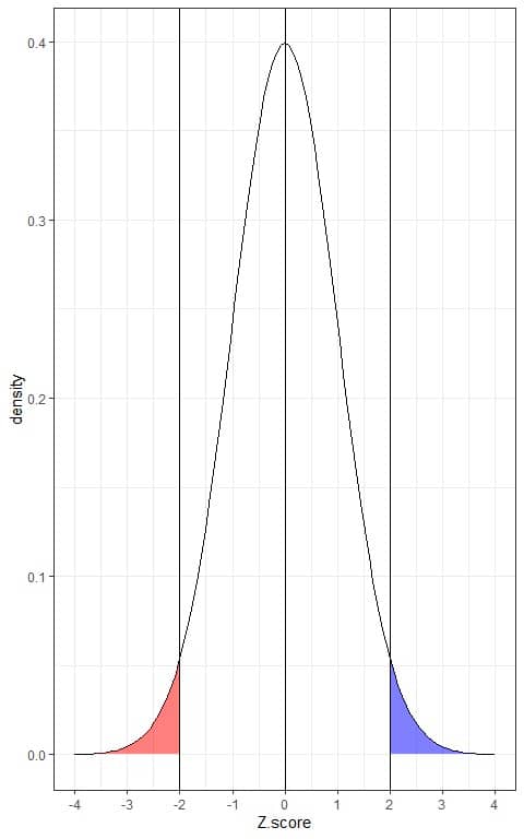
The blue shaded area = probability that the data has a Z-score more than 2 = 0.025 or 2.5%.

The red shaded area = probability that the data has a Z-score less than -2 = 0.025 or 2.5%.

• The probability of data that are larger than 3 standard deviations from the mean= the probability of data that are smaller than 3 standard deviations from the mean= 0.0015 or 0.15%.

This means that 0.15% of the population has Z-score more than 3 and another 0.15% of the population has Z-score smaller than -3.

In other words, the probability of data from this population to have more than 3 Z-score = the probability of data from this population to have less than -3 Z-score = 0.15%.

Both are negligible quantities.

This is plotted as follows:

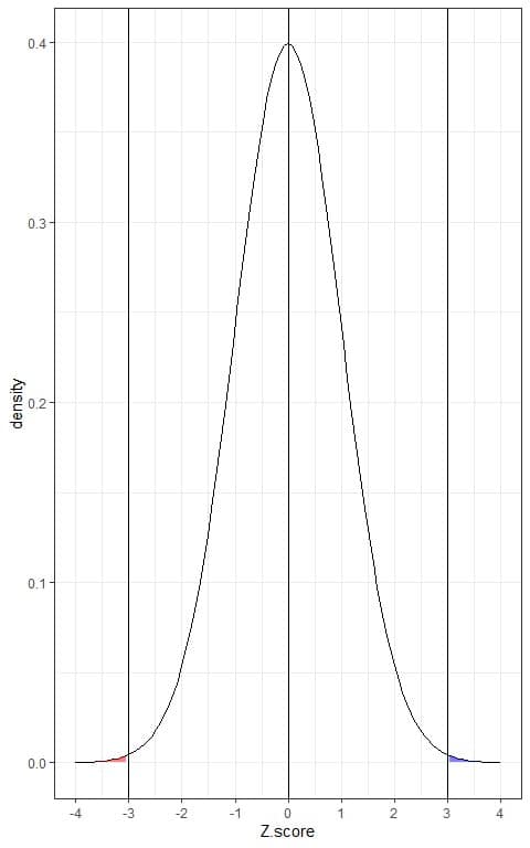
The blue shaded area = probability that the data has a Z-score more than 3 = 0.0015 or 0.15%.

The red shaded area = probability that the data has a Z-score less than -3 = 0.0015 or 0.15%.

4. How to calculate Z-score?

We will calculate the Z-score using the above formula.

The above probabilities correspond (approximately) to the real probabilities that we observe in our data if the data follows the shape of a normal distribution.

– Example 1

The following is the relative frequency table and histogram for heights (in cm) from a certain population.

The mean height of this population = 163 cm and standard deviation = 9 cm.

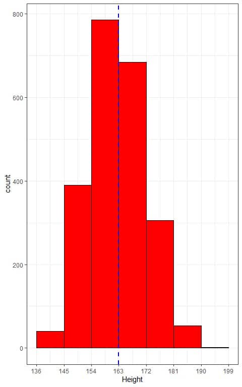
The histogram of heights from this population can be approximated by the normal distribution because the distribution is nearly symmetric around the mean (163 cm, blue dashed line) and bell-shaped.

In that case, we will convert all the data values in the range column to a Z-score value as follows:

• The Z-score for 136 cm height = (136-163)/9 = -3.
• The Z-score for 145 cm height = (145-163)/9 = -2.
• The Z-score for 154 cm height = (154-163)/9 = -1.
• The Z-score for 163 cm height = (163-163)/9 = 0.
• The Z-score for 172 cm height = (172-163)/9 = 1.
• The Z-score for 181 cm height = (181-163)/9 = 2.
• The Z-score for 190 cm height = (190-163)/9 = 3.
• The Z-score for 199 cm height = (199-163)/9 = 4.

Then, we add the range (in terms of Z-score values to our table):

We will see how the 68-95-99.7% rule give results that are similar to the actual proportion of heights in this population:

• 68% of the data have Z-score between -1 and +1.

The observed proportion for the data within -1 and +1 Z-score = relative frequency of range “-1-0” + relative frequency of range “0-1” = 0.35+0.30 = 0.65 or 65%.

• 95% of the data have Z-score between -2 and +2.

The observed proportion for the data within -2 and +2 Z-score= sum of relative frequencies for ranges between“-2-2” =0.17+ 0.35+0.30+0.14 = 0.96 or 96%.

• 99.7% of the data have Z-score between -3 and +3.

The observed proportion for the data within -3 and +3 Z-score= sum of relative frequencies for ranges between“-3-3” =0.02+0.17+ 0.35+0.30+0.14+0.02 = 1 or 100%.

5. The role of Z-score

1. Compare different data points within the same normal distribution.
2. Compare different data points that are from different normal distributions.

– Example: Comparing different data points within the same normal distribution

The weight from a certain population follows the normal distribution curve with a mean = 73 kg and standard deviation = 13 kg.

Two friends, Mark and Sam, have weights of 86 and 60 Kg respectively. Although it is clear that Mark has a heavier weight than Sam. How do these individuals compare to the general population weights?

• Calculate the Z-score for each weight value:

The Z-score for Mark’s weight of 86 kg = (86-mean)/standard deviation = (86-73)/13 = 1.

The Z-score of Mark’s weight = 1. This means that his weight is 1 standard deviation more than the mean weight in this population.

The Z-score for Sam’s weight of 60 kg = (60-mean)/standard deviation = (60-73)/13 = -1.

The Z-score of Sam’s weight = -1. This means that his weight is 1 standard deviation below the mean weight in this population.

This can be plotted as follows:

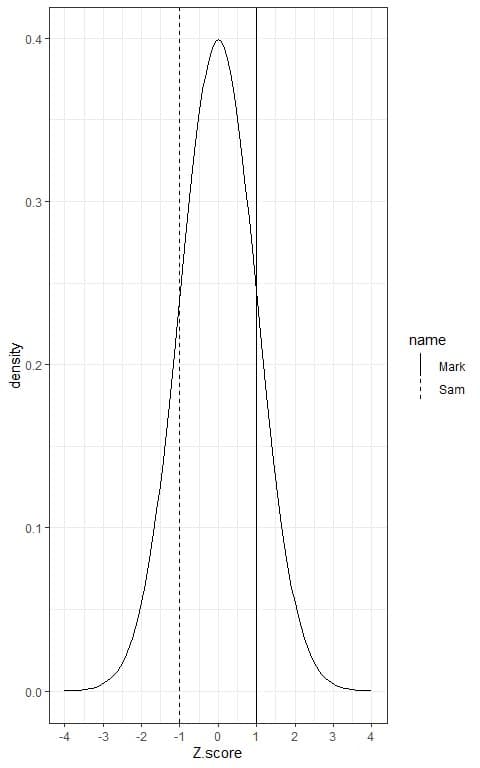
The solid black line is the Z-score for Mark’s weight, while the dashed line is the Z-score for Sam’s weight.

• From the properties of Z-score, 16% of the population have Z-score more than 1 and another 16% of the population have Z-score smaller than -1.

This means that 16% of the population has weights more than Mark’s weight because his Z-score = 1. This also means that 100-16 = 84% of the population have weights less than Mark’s weight.

On the other hand, 16% of the population has weights less than Sam’s weight because his Z-score = -1. This also means that 100-16 = 84% of the population have weights more than Sam’s weight.

For Mark’s weight, this can be plotted as follows:

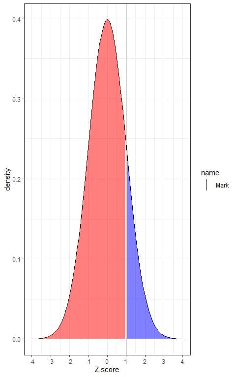
The blue shaded area = probability that the population has a Z-score or weight more than Mark’s weight or more than 1 = 0.16 or 16%.

The red shaded area = probability that the population has a Z-score or weight less than Mark’s weight or less than 1 = 0.84 or 84%.

For Sam’s weight, this can be plotted as follows:

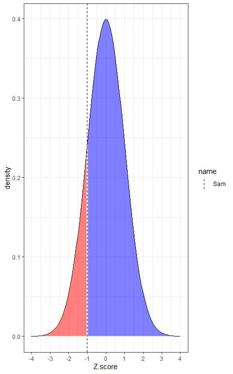
The blue shaded area = probability that the population has a Z-score or weight more than Sam’s weight or more than -1 = 0.84 or 84%.

The red shaded area = probability that the population has a Z-score or weight less than Sam’s weight or less than -1 = 0.16 or 16%.

In conclusion:

• Mark’s weight is the 84% percentile of the data because 84% of the data have weights less than his weight.
• Sam’s weight is the 16% percentile of the data because 16% of the data have weights less than his weight.

– Example: Comparing different data points that are from different normal distributions

The weight from a certain population follows the normal distribution curve with a mean = 73 kg and standard deviation = 13 kg.

On the other hand, the height from the same population also follows the normal distribution curve with a mean = 163 cm and standard deviation = 9 cm.

A person from this population, called Sam, has a weight of 60 Kg and a height of 163 cm.

How does Sam’s weight and height compare to the general population weights and heights?

1. Plot the weight and height of Sam in their respective normal distribution.

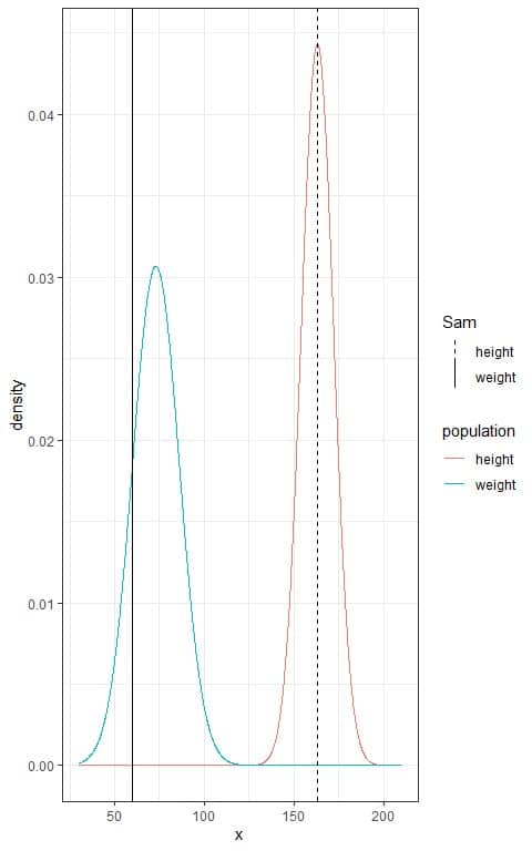
We see that:

• The blue population weight curve is bell-shaped, symmetric, and peaked at its mean = 73 kg.
• The red population height curve is bell-shaped, symmetric, and peaked at its mean = 163 cm.
• Sam’s weight (60 kg) is plotted as a solid vertical line to the left of the population weight peak because it is lower than the population mean weight = 73 kg.
• Sam’s height is plotted as a dashed vertical line at the peak of the population height because it is equal to the population mean height = 163 cm.

2. Calculate the Z-score for each value:

The Z-score for Sam’s weight of 60 kg = (60-mean)/standard deviation = (60-73)/13 = -1.

The Z-score of Sam’s weight = -1. This means that his weight is 1 standard deviation less than the mean weight in this population.

The Z-score for Sam’s height of 163 cm = (163-mean)/standard deviation = (163-163)/9 = 0.

The Z-score of Sam’s height = 0. This means that his height is equal to the mean height in this population.

This can be plotted as follows:

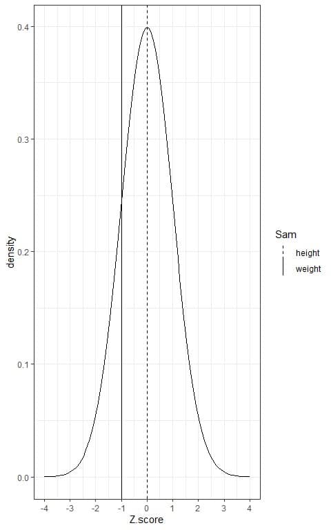
We see that:

• The Z-score standardizes the distribution of population weight and height to become a standard normal distribution with mean = 0 and standard deviation = 1.
• The solid vertical line is the Z-score for Sam’s weight, while the dashed line is the Z-score for Sam’s height.
• As the two lines are within the same distribution, so we now can compare between them.

If we dashed the area below each line, we will get the following figure:

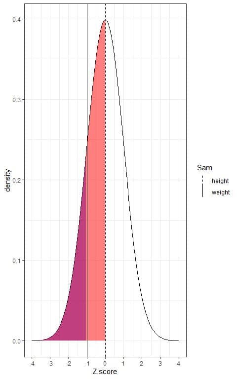
We see that:

• The area below the dashed line is larger than the area that is below the solid line.
• This means that the population percentage that has heights lower than Sam’s height is higher than the population percentage that has weights less than Sam’s weight.

3. From the properties of Z-score, 50% of the population have Z-score smaller than 0, while 16% of the population have Z-score smaller than -1.

This means that 50% of the population have heights less than Sam’s height or 50% of the population have heights more than Sam’s height.

On the other hand, 16% of the population have weights less than Sam’s weight or 84% of the population have weights more than Sam’s weight.

In conclusion:

• Sam’s height is the 50% percentile of the data because 50% of the data (or the population) have heights less than his height.
• Sam’s weight is the 16% percentile of the data because 16% of the data (or the population) have weights less than his weight.

6. Practice questions

1. The Grade point average (GPA) for a sample of students follows the normal distribution curve with a mean = 3.6 and standard deviation = 0.3.

One student has a GPA value of 3.9. How does this student compare to other students?

2. The Grade point average (GPA) for a sample of students from a certain class (class1) follows the normal distribution curve with a mean = 2.5 and standard deviation = 0.5.

In another class (class2), the GPA follows the normal distribution curve with a mean = 3.2 and standard deviation = 0.4.

A student from class1 has a GPA value of 3.5.

Another student from class2 has a GPA value of 3.6.

Which student is doing better relative to the GPA values of his class?

3. The following plot shows the normal distributions for the wind speed of a sample of two types of storms, hurricane and tropical storms.

Alex is a hurricane storm and its wind speed is plotted as a solid vertical line.

Zeta is a tropical storm and its wind speed is plotted as a dashed vertical line.

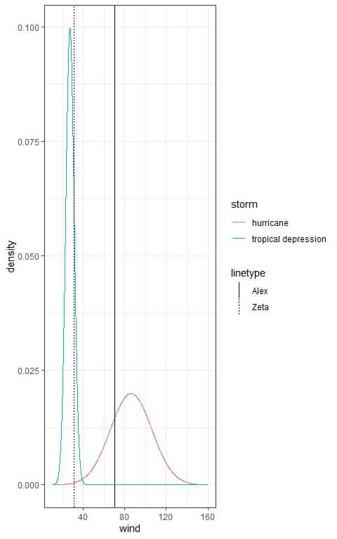
Which storm is worst relative to its class?

4. The following table lists the mean and standard deviation of the weights of diamonds per their quality of cut.

One diamond has a “Fair” cut that weighed 2.00 grams, while another diamond has an “Ideal” cut that weighed 1.5 grams.

Assuming that the weights for each cut follow a normal distribution, what is the Z-score for each diamond?

5. The following table lists the mean and standard deviation of the ozone values per their month of measurement.

An ozone measurement in May (month = 5) was 24.5, while an ozone measurement in June (month = 6) was 28.5.

Assuming that the ozone measurements for each month follow a normal distribution, what is the Z-score for each ozone value?

7. Answer key

1. Calculate the Z-score for the student GPA value:

The Z-score = (3.9-mean)/standard deviation = (3.9-3.6)/0.3 = 1.

From the properties of the Z-score, 16% of the population (or our sample) have Z-score more than 1.

This means that 16% of our sample have GPA values more than that student.

This also means that 100-16 = 84% of our sample have GPA values less than that student.

The student’s GPA value is the 84% percentile because 84% of the students in our sample have GPA values less than him.

2. Although student from class2 has a higher GPA, we should standardize both distributions so they can be compared to each other.

• Calculate the Z-score for each student’s GPA value:

For student from class1, the Z-score = (3.5-mean)/standard deviation = (3.5-2.5)/0.5 = 2.

For student from class2, the Z-score = (3.6-mean)/standard deviation = (3.6-3.2)/0.4 = 1.

• From the properties of the Z-score, 16% of the population (or our sample) have Z-score more than 1.

Also, 2.5% of the population (or our sample) have a Z-score of more than 2.

For the student from class1 with Z-score = 2, only 2.5% of the students from class1 have GPA values more than him.

This means that this student is doing better than 97.5% of the students from class1.

For the student from class2 with Z-score = 1, 16% of the students from class2 have GPA values more than him.

This means that this student is doing better than 84% of the students from class2.

The student from class1 is doing better because he gets a GPA value that is better than 97.5% of his classmates, while the student from class2 has a GPA value that is better than only 84% of his classmates.

In other words, the student from class1 is doing better because he has a larger Z-score.

3. Alex storm has higher wind speed and Zeta storm has lower wind speed.

However, the Alex wind speed is below the peak of the hurricane normal distribution, while Zeta wind speed is above the peak of the tropical depression normal distribution.

Alex storm is worse (higher) in its wind speed relative to tropical depression storms than Zeta wind speed relative to hurricane storms.

4. Calculate the Z-score for each diamond weight:

For the diamond with “Fair” cut, the Z-score = (2.00-mean)/standard deviation = (2.00-1.05)/0.52 = 1.83.

For the diamond with “Ideal” cut, the Z-score = (1.5-mean)/standard deviation = (1.5-0.7)/0.43 = 1.86.

5. Calculate the Z-score for each ozone value:

For the ozone measured in May, the Z-score = (24.5-mean)/standard deviation = (24.5-23.62)/22.22 = 0.04.

For the ozone measured in June, the Z-score = (28.5-mean)/standard deviation = (28.5-29.44)/18.21 = -0.05.

Although the ozone value in June was higher than that in May, the Z-score of the value measured in June was lower than that measured in May.

Previous Lesson | Main Page | Next Lesson