ANOVA Test – Explanation & Examples

The definition of the one-way analysis of variance (ANOVA) test is:

“The ANOVA test compares the means of two or more groups to see if there is a difference between them.”

In this topic, we will discuss the one-way ANOVA test from the following aspects:

1. What is an ANOVA test?
2. Hypothesis testing for the one-way ANOVA test.
3. When to use an ANOVA test?
4. How to do an ANOVA test?
5. Practice questions.
6. Answer key.

1. What is an ANOVA test?

The one-way analysis of variance (ANOVA) is used to determine whether there are any statistically significant differences between the means of a numerical variable from two or more groups.

Example of two group comparison

One study considered all pregnancies between 1960 and 1967 among women in the Kaiser Foundation Health Plan in the San Francisco East Bay area.

The goal is to model the weight of the infants (bwt, in ounces) using variables including length of pregnancy in days (gestation), mother’s age in years (age), mother’s height in inches (height), whether the child was the first-born (parity), mother’s pregnancy weight in pounds (weight), and whether the mother was a smoker (smoke).

We want to test whether there are any statistically significant differences between the means of infants’ weights (numerical variable) from smoker and non-smoker mothers (two groups).

We can look at the infants’ weight means from the following table:

We see that:

• When smoke = 0, this means non-smoking mothers, and when smoke = 1, this means smoking mothers.
• The infants’ mean weight for non-smoking mothers is 123.05 which is higher than that for the smoking mothers which is 114.11.
• We want to test if the two groups are truly different in their infants’ birth weight.

We can also look at the data in the following box plots:

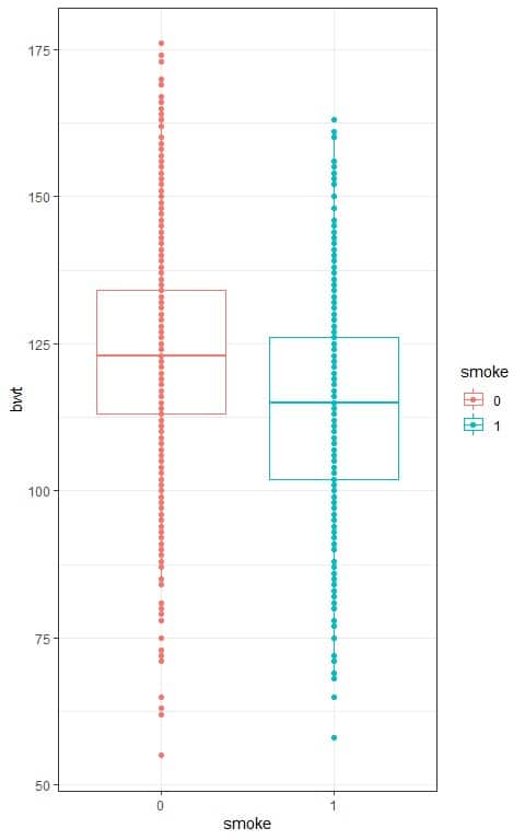
We see that:

• The x-axis is the smoking categories, 0 = non-smoking mothers and 1 = smoking mothers.
• The y-axis is the infant birth weight (bwt).
• The median line (central line) of the box plot for non-smoking mothers is higher than that for smoking mothers.
• The median nearly equals the mean for normally distributed variables. From the above table, we see that the mean of non-smoking mothers is higher than that of smoking mothers.
• The points representing the birth weight for non-smoking mothers (red points) tend to be higher than the points representing the birth weight for smoking mothers (blue points).

Example of three group comparison

The Results from the US Census American Community Survey, 2012 showed the following table for the income means per education level:

We see that:

• The mean income for high school or lower (hs or lower) education persons is 14092.83 which is lower than the mean income for college persons (35330.84) and the mean income for graduated (grad) persons (68298.82).
• We want to test whether there are any statistically significant differences between the means of income (numerical variable) across the 3 groups of education levels, high school or lower, college, and graduated.

We can also look at the data in the following box plots:

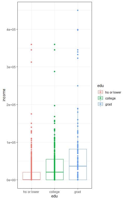
We see that:

• The x-axis is the education level categories, high school or lower, college, and graduated.
• The y-axis is the income values.
• The median line (central line) of the box plot for graduated persons is higher than that for college persons, which in turn is higher than the median line for high school or lower persons.
• The median nearly equals the mean for normally distributed variables. From the above table, we see that the mean income of graduated persons is higher than that for college persons, which in turn, is higher than the mean income for high school or lower persons.

2. Hypothesis testing for the one-way ANOVA test

We start with two exclusive possibilities for the unknown truth. Then, use the sample to choose between these two possibilities for the truth.

The two possibilities are the Null hypothesis, Ho, and the Alternative hypothesis, Ha.

Hypothesis testing is denoted as:

• Ho: μ_1=μ_2=μ_3=…..=μ_k.

Where:

µ = group mean and k = number of groups.

The mean of each of the groups is the same and the observed difference was due to chance.

• Ha: there are at least two group means that are statistically significantly different from each other.

When the groups are larger than 2 groups, the one-way ANOVA test cannot tell you which specific groups were statistically significantly different from each other.

To determine which specific groups differed from each other, you need to use a post hoc test.

3. When to use an ANOVA test?

Three main conditions must be met to do the ANOVA test:

1. The numerical variable is normally distributed in each group that is being compared. For example, When we are comparing two groups (smoking and non-smoking mothers) on their infant birth weight, the infant birth weight values should be normally distributed in the smoking group as well as in the non-smoking group.
2. The variance within each group must be equal.
3. The observations are independent within and across groups.

This means that there is no pairing of your data. For example, you cannot compare the mean test score for students before and after taking a test preparation course because you are comparing the same group on two occasions.

4. How to do an ANOVA test?

We will go through several examples.

– Example 1

The following table is the results from an experiment to compare yields (numerical variable) obtained under a control (ctrl) and a treatment (trt1) condition.

Source: Dobson, A. J. (1983) An Introduction to Statistical Modelling. London: Chapman and Hall.

We see that there are 10 yield measurements for each group with a total of 20 measurements.

We can also look at the data in the following box plots:

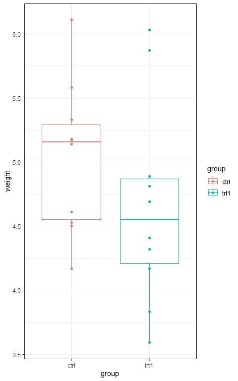
We see that:

• The x-axis is the group categories, “ctrl” for control and “trt1” for treatment.
• The y-axis is the yield (measured by the dried weight of plants).
• The median line (central line) of the box plot for the “ctrl” group is higher than that for the “trt1” group.

We will follow these steps:

1. Calculate the group means and the overall mean.

The “ctrl” mean = (4.17+ 5.58+ 5.18+ 6.11+ 4.50+ 4.61+ 5.17+ 4.53+ 5.33+ 5.14)/10 = 5.03.

The “trt1” mean = (4.81+ 4.17+ 4.41+ 3.59+ 5.87+ 3.83+ 6.03+ 4.89+ 4.32+ 4.69)/10 = 4.66.

The overall mean = sum of all data/number of data = (4.17+ 5.58+ 5.18+ 6.11+ 4.50+ 4.61+ 5.17+ 4.53+ 5.33+ 5.14+4.81+ 4.17+ 4.41+ 3.59+ 5.87+ 3.83+ 6.03+ 4.89+ 4.32+ 4.69)/20 = 4.85.

2. Calculate the between-group variability or the between the sum of squares (BSS).

The BSS represents the deviation of a group mean from the overall mean and is an indication of between-group variability.

The BSS is calculated using the following formula:

BSS=∑n_j (x_j-x)^2

where:

∑: a greek symbol that means “sum”.

n_j: the sample size of group j.

x_j: the mean of group j.

x: the overall mean.

In our example, we have two groups so we sum two quantities to get the BSS.

The BSS = 10(5.03-4.85)^2 + 10(4.66-4.85)^2 = 0.685.

3. Calculate the within-group variability or the within the sum of squares (WSS).

The WSS represents the deviation of an individual observation from the group mean for that observation and is an indication of within-group variability.

We calculate WSS using the standard deviation (or the variance) and the sample size of each group using the following formula:

WSS=∑(n_j-1)s_j^2

where:

n_j: the sample size of group j.

s_j: the standard deviation of group j.

In our example, we have two groups so we sum two quantities to get the WSS.

The standard deviation for the “ctrl” group = 0.583.

The standard deviation for the “trt1” group = 0.794.

The WSS = 9(0.583)^2 + 9(0.794)^2 = 8.733.

4. Calculate the total variability in the data or the total sum of squares (TSS).

TSS = BSS + WSS.

In our example, TSS = 0.685 + 8.733 = 9.418.

5. Calculate the between mean square (BMS) and within mean square (WMS).

BMS=BSS/(k-1)

WMS=WSS/(n-k)

where:

k = number of groups.

n = total number of data.

In our example, k = 2 and n = 20.

BMS = 0.685/(2-1) = 0.685.

WMS = 8.733/(20-2) = 8.733/18 = 0.485.

6. Compute the F-value which is the ratio between BMS and WMS.

F-value = BMS/WMS = 0.685/0.485 = 1.41.

7. If the null hypothesis is true, the F-value has an F distribution with degrees of freedom or df1 = k-1 and df2 = n-k.

In our example, df1 = 2-1=1 and df2 = 20-2 = 18.

8. The p-value is given by the area to the right of the F-value under this F distribution.

The following is the F distribution with 1 df1 and 18 df2.

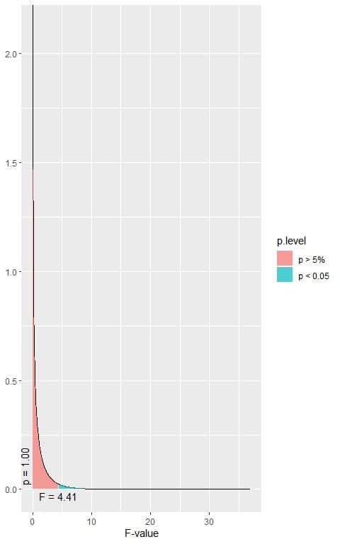
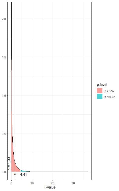The total area under the curve is 1.00 or 100%.

In the first plot, we see that when the F-value = 4.41, the area to the right or the p-value < 0.05.

In our example, the F-value = 1.41 (plotted as a vertical line in the second plot), so the p-value is larger than 0.05.

9. Make a decision, accept Ha, or fail to reject Ho.

The p-value is > 0.05, so it is a statistically non-significant result and we fail to reject the null hypothesis. This means that there is no difference between the mean yield of the 2 groups (“ctrl” and “trt1”) and the observed difference was due to chance or sampling error.

– Example 2

One study considered all pregnancies between 1960 and 1967 among women in the Kaiser Foundation Health Plan in the San Francisco East Bay area.

We want to test if there is any difference between the mean of infants’ weights (numerical variable) from smoker and non-smoker mothers (two groups).

We can look at the infants’ weight means, standard deviations, and the sample size for the two groups in the following table:

We see that:

• When smoke = 0, this means non-smoking mothers, and when smoke = 1, this means smoking mothers.
• The infants’ mean weight for non-smoking mothers is 123.05 which is higher than that for the smoking mothers which is 114.11.
• The standard deviation for the weights in the non-smoking group is 17.4, while the standard deviation for the smoking group is 18.1.
• The sample size for the non-smoking group is 742, while the sample size for the smoking group is 484.

The total sample in our data = 742+484 = 1226.

We will follow these steps:

1. Calculate the group means and the overall mean.

The group means are already calculated.

To calculate the overall mean from the groups means:

x=(∑n_j x_j)/n

where:

∑: a greek symbol that means “sum”.

n_j: the sample size of group j.

x_j: the mean of group j.

x: the overall mean.

n: the total sample size.

The overall mean = ((mean of group 1 X sample size of group 1) + (mean of group 2 X sample size of group 2))/number of data = ((123.05 X 742)+(114.11 X 484))/1226 = 119.52.

2. Calculate the between-group variability or the between the sum of squares (BSS).

In our example, we have two groups so we sum two quantities to get the BSS.

The BSS = 742(123.05-119.52)^2 + 484(114.11-119.52)^2 = 23411.75.

3. Calculate the within-group variability or the within the sum of squares (WSS).

In our example, we have two groups so we sum two quantities to get the WSS.

The WSS = (742-1)(17.4)^2 + (484-1)(18.1)^2 = 382580.8.

4. Calculate the total variability in the data or the total sum of squares (TSS).

TSS = BSS + WSS.

In our example, TSS = 23411.75 + 382580.8 = 405992.5.

5. Calculate the between mean square (BMS) and within mean square (WMS).

In our example, k = number of groups = 2 and n = total sample size = 1226.

BMS = 23411.75/(2-1) = 23411.75.

WMS = 382580.8/(1226-2) = 312.57.

6. Compute the F-value which is the ratio between BMS and WMS.

F-value = BMS/WMS = 23411.75/312.57 = 74.90.

7. If the null hypothesis is true, the F-value has an F distribution with degrees of freedom or df1 = k-1 and df2 = n-k.

In our example, df1 = 2-1=1 and df2 = 1226-2 = 1224.

8. The p-value is given by the area to the right of the F-value under this F distribution.

The following is the F distribution with 1 df1 and 1224 df2.

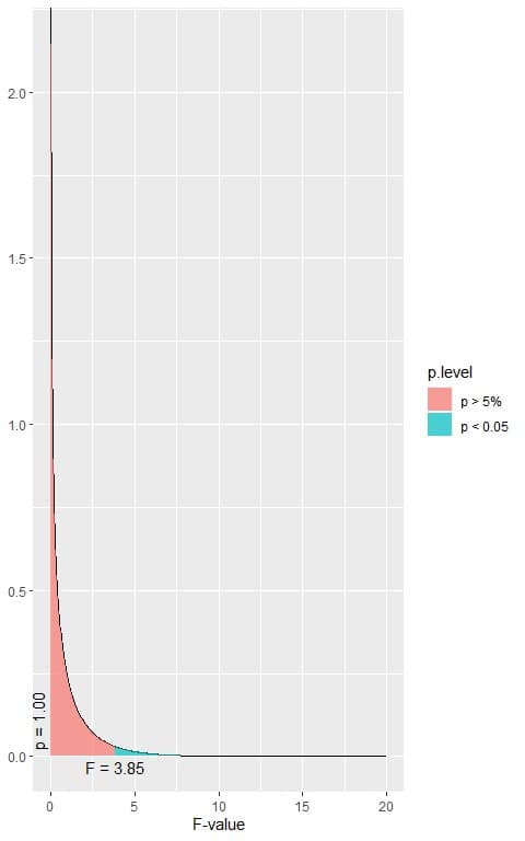
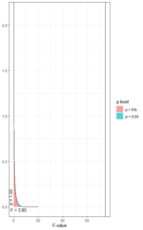
In the first plot, when the F-value = 3.85, the area to the right or the p-value < 0.05.

In our example, the F-value = 74.90 (plotted as a vertical line in the second plot), so the p-value is very much smaller than 0.05.

9. Make a decision, accept Ha, or fail to reject Ho.

The p-value is < 0.05, so it is a statistically significant result and we reject the null hypothesis. This means that there is a difference between the mean birth weight of the 2 groups (smoking and non-smoking).

We have only two groups in our example, so we can conclude that the infant birth weight of non-smoking mothers is higher than the infant birth weight of smoking mothers on average.

– Example 3

The Results from the US Census American Community Survey, 2012 showed the following table for the income means per education level:

We see that:

• The mean income for high school or lower (hs or lower) education persons is 14092.83 which is lower than the mean income for college persons (35330.84) and the mean income for graduated (grad) persons (68298.82).
• The standard deviation for the income in the high school or lower education persons is 27715.59, while the standard deviation for the income in the college persons is 46785.23 and the standard deviation for the income for graduated persons is 100202.50.
• The sample size for the high school or lower education group is 1120, while the sample size for the college group is 359 and the sample size for the graduated group is only 144.

The total sample in our data = 1120+359+144 = 1623.

We want to test whether there are any statistically significant differences between the means of income (numerical variable) across the 3 groups of education levels, high school or lower, college, and graduated, assuming that all ANOVA assumptions are met.

Note: In fact, the variance within each group is not equal as we see from the great variability of standard deviations of the 3 groups, but for simplicity, we assume that they are equal to show the calculations.

We will follow these steps:

1. Calculate the group means and the overall mean.

The group means are already calculated.

To calculate the overall mean from the groups mean:

The overall mean = ((mean of group 1 X sample size of group 1) + (mean of group 2 X sample size of group 2) + (mean of group 3 X sample size of group 3))/number of data = ((14092.83 X 1120)+(35330.84 X 359)+(68298.82 X 144))/1623 = 23599.98.

2. Calculate the between-group variability or the between the sum of squares (BSS).

In our example, we have 3 groups so we sum 3 quantities to get the BSS.

The BSS = 1120(14092.83-23599.98)^2 + 359(35330.84-23599.98)^2 + 144(68298.82-23599.98)^2 = 438345330481.

3. Calculate the within-group variability or the within the sum of squares (WSS).

In our example, we have 3 groups so we sum 3 quantities to get the WSS.

The WSS = (1120-1)(27715.59)^2 + (359-1)(46785.23)^2 + (144-1)(100202.50)^2 = 3078972683621.

4. Calculate the total variability in the data or the total sum of squares (TSS).

TSS = BSS + WSS.

In our example, TSS = 438345330481 + 3078972683621 = 3517318014102.

5. Calculate the between mean square (BMS) and within mean square (WMS).

In our example, k = number of groups = 3 and n = total sample size = 1623.

BMS = 438345330481/(3-1) = 219172665241.

WMS = 3078972683621/(1623-3) = 1900600422.

6. Compute the F-value which is the ratio between BMS and WMS.

F-value = BMS/WMS = 219172665241/1900600422 = 115.32.

7. If the null hypothesis is true, the F-value has an F distribution with degrees of freedom or df1 = k-1 and df2 = n-k.

In our example, df1 = 3-1=2 and df2 = 1623-3 = 1620.

8. The p-value is given by the area to the right of the F-value under this F distribution.

The following is the F distribution with 2 df1 and 1620 df2.

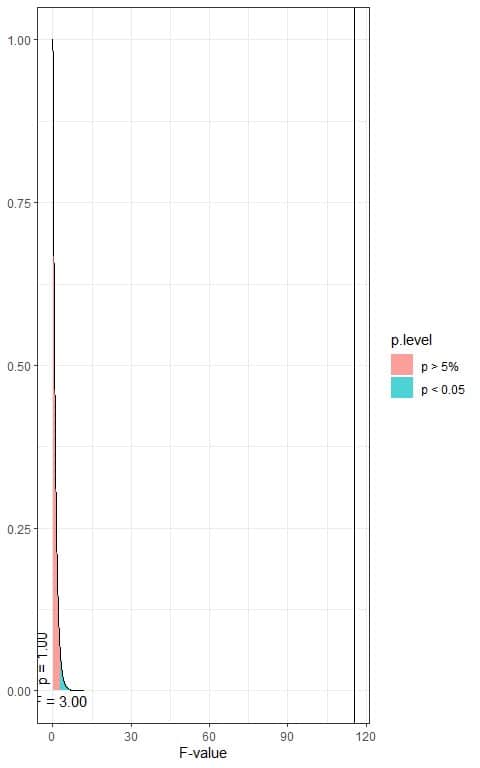
In the first plot, when the F-value = 3.00, the area to the right or the p-value < 0.05.

In our example, the F-value = 115.32 (plotted as a vertical line in the second plot), so the p-value is very much smaller than 0.05.

9. Make a decision, accept Ha, or fail to reject Ho.

The p-value is < 0.05, so it is a statistically significant result and we reject the null hypothesis. This means that there is a difference between at least two of the means.

We have 3 groups in our example, so we cannot know which pair mean is significantly different from each other, The 3 possible pairs are:

1. Mean income of high school education vs. mean income of college education.
2. Mean income of high school education vs. mean income of graduated education.
3. Mean income of college education vs. mean income of graduated education.

– Example 4

A Survey of Duke students showed the following table for the means of Grade point average (GPA) per their academic major:

We see that:

• The mean GPA for students with arts and humanities major is 3.57 which is lower than the mean GPA for natural sciences students (3.62) and the mean mean GPA for social sciences students (3.59).
• The standard deviation for GPA of students with arts and humanities major is 0.26, while the standard deviation for GPA of natural sciences students is 0.29 and the standard deviation for GPA of natural sciences students is 0.30.
• The sample size for the arts and humanities major group is 33, while the sample size for the natural sciences major group is 53 and the sample size for the social sciences group is 114.

The total sample in our data = 33+53+114 = 200.

We want to test whether there are any statistically significant differences between the means of GPA (numerical variable) across the 3 groups of academic majors, arts and humanities, natural sciences, and social sciences, assuming that all ANOVA assumptions are met.

We can see the individual GPA values in the following box plots:

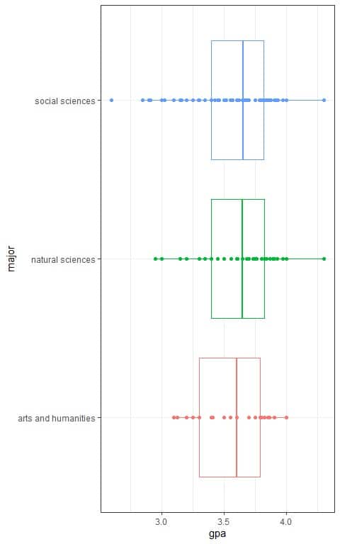
We see that the median lines for the natural sciences and social sciences major are slightly higher than the median line for the arts and humanities major.

We will follow these steps:

1. Calculate the group means and the overall mean.

The group means are already calculated.

To calculate the overall mean from the groups mean:

The overall mean = ((mean of group 1 X sample size of group 1) + (mean of group 2 X sample size of group 2) + (mean of group 3 X sample size of group 3))/number of data = ((3.57 X 33)+(3.62 X 53)+(3.59 X 114))/200 = 3.59.

2. Calculate the between-group variability or the between the sum of squares (BSS).

In our example, we have 3 groups so we sum 3 quantities to get the BSS.

The BSS = 33(3.57-3.59)^2 + 53(3.62-3.59)^2 + 114(3.59-3.59)^2 = 0.0609.

3. Calculate the within-group variability or the within the sum of squares (WSS).

In our example, we have 3 groups so we sum 3 quantities to get the WSS.

The WSS = (33-1)(0.26)^2 + (53-1)(0.29)^2 + (114-1)(0.30)^2 = 16.7064.

4. Calculate the total variability in the data or the total sum of squares (TSS).

TSS = BSS + WSS.

In our example, TSS = 0.0609 + 16.7064 = 16.7673.

5. Calculate the between mean square (BMS) and within mean square (WMS).

In our example, k = number of groups = 3 and n = total sample size = 200.

BMS = 0.0609/(3-1) = 0.03045.

WMS = 16.7064/(200-3) = 0.08480406.

6. Compute the F-value which is the ratio between BMS and WMS.

F-value = BMS/WMS = 0.03045/0.08480406 = 0.359.

7. If the null hypothesis is true, the F-value has an F distribution with degrees of freedom or df1 = k-1 and df2 = n-k.

In our example, df1 = 3-1=2 and df2 = 200-3 = 197.

8. The p-value is given by the area to the right of the F-value under this F distribution.

The following is the F distribution with 2 df1 and 197 df2.

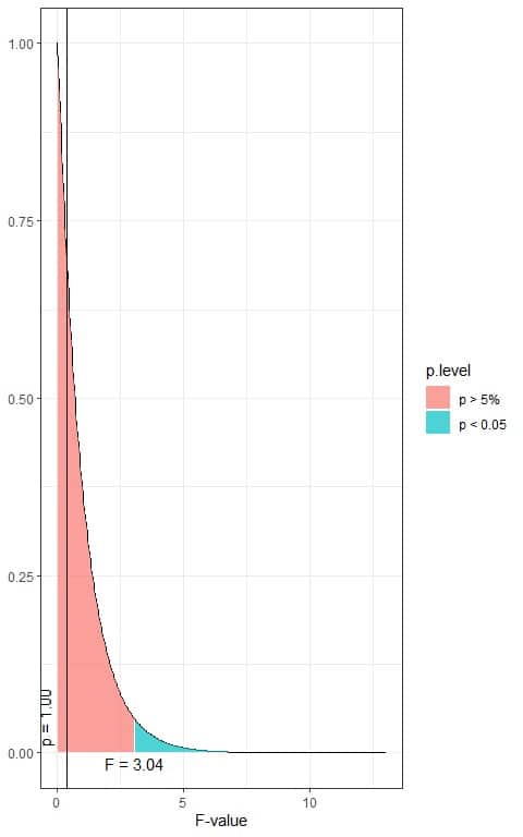
In the first plot, when the F-value = 3.04, the area to the right or the p-value < 0.05.

In our example, the F-value = 0.359 (plotted as a vertical line in the second plot), so the p-value is larger than 0.05.

9. Make a decision, accept Ha, or fail to reject Ho.

The p-value is > 0.05, so it is a statistically non-significant result and we fail to reject the null hypothesis. This means that there is no difference between the group means.

All the 3 major groups have equivalent GPAs on average.

5. Practice questions

1. The NOAA Atlantic hurricane database best track data showed the following table for the means of storm’s maximum sustained wind speed (in knots) per Saffir-Simpson storm category (from -1 to 5):

We want to test whether there are any statistically significant differences between the means of wind speed (numerical variable) across the storm categories, assuming that all ANOVA assumptions are met.

F-value = 25996.

The following is the F distribution with 6 df1 and 10003 df2 that corresponds to the null hypothesis.

2. The following box plots show the distribution of HDL cholesterol (hdl) in males and females from a certain survey.

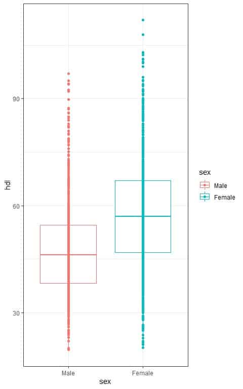
The calculated F-value = 284.86.

The following is the F distribution with 1 df1 and 2223 df2 that corresponds to the null hypothesis.

Are there any statistically significant gender differences in the means of hdl, assuming that all ANOVA assumptions are met?

3. The following box plots show the distribution of body mass index (bmi) per smoking status (smoke) from a certain survey.

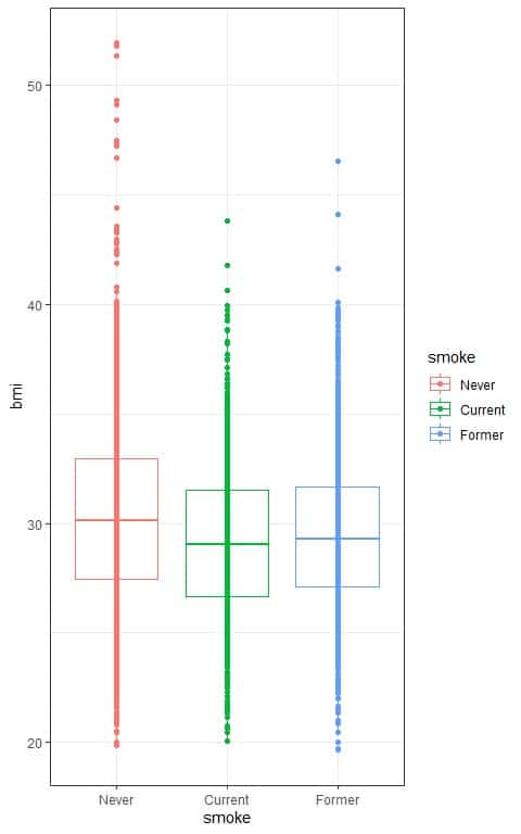
The calculated F-value = 46.111.

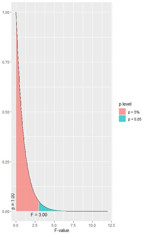
The following is the F distribution with 2 df1 and 6321 df2 that corresponds to the null hypothesis.

Are there any statistically significant differences in the means of bmi between the different smoking groups, assuming that all ANOVA assumptions are met?

4. The following box plots show the distribution of daily solar radiation values (Solar.R) per month of measurement (Month) in New York, May to September 1973.

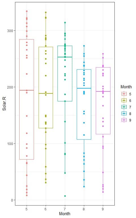
The calculated F-value = 1.4306.

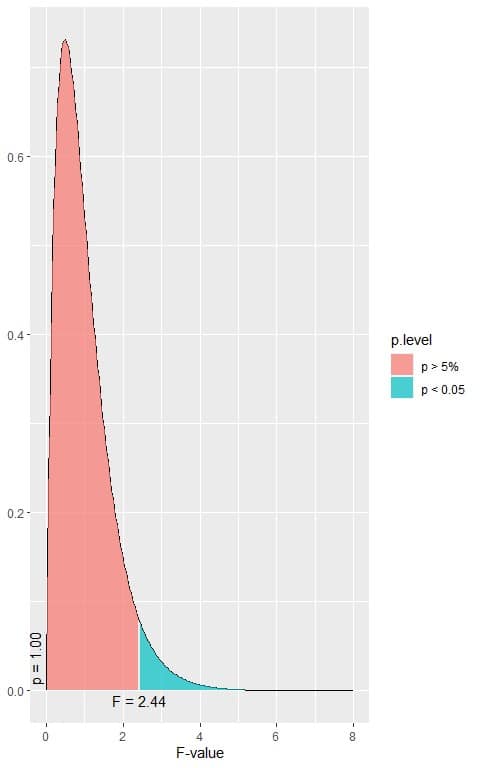
The following is the F distribution with 4 df1 and 141 df2 that corresponds to the null hypothesis.

Is there any statistically significant difference in the mean of solar measurement between the different months, assuming that all ANOVA assumptions are met?

5. The following box plots show the distribution of Sepal.Length values (Sepal.Length) for each of 3 species of iris. The species are Iris setosa, versicolor, and virginica.

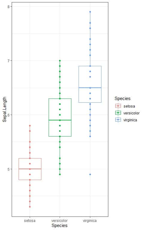
The calculated F-value = 119.26.

The following is the F distribution with 2 df1 and 147 df2 that corresponds to the null hypothesis.

Is there any statistically significant difference in the mean of Sepal.Length between the 3 species, assuming that all ANOVA assumptions are met?

6. Answer key

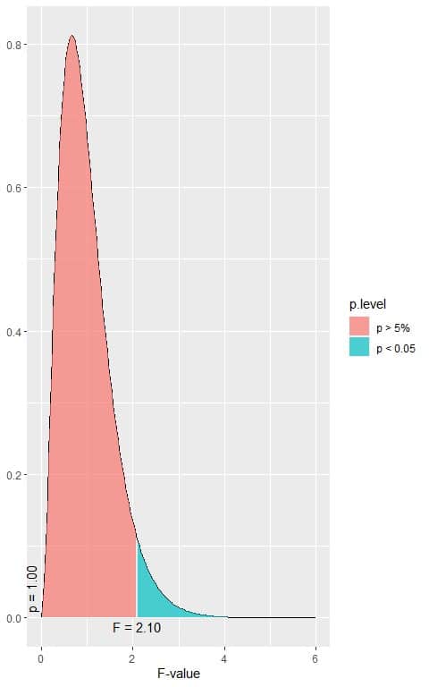
1. When the F-value = 2.10, the area to the right or the p-value < 0.05.

In our example, the F-value = 25996 which is larger than 2.10, so the p-value is very much smaller than 0.05.

The p-value is < 0.05, so it is a statistically significant result and we reject the null hypothesis.

This means that there is a difference between at least two of the categories’ means.

We have 7 groups in our data, so we cannot know which pair mean is significantly different from each other.

2. When the F-value = 3.85, the area to the right or the p-value < 0.05.

In our example, the F-value = 284.86 which is larger than 3.85, so the p-value is very much smaller than 0.05.

The p-value is < 0.05, so it is a statistically significant result and we reject the null hypothesis.

We have only two groups in our data, so we can conclude that, in this population, the hdl of females is higher than the hdl of males on average.

3. When the F-value = 3.00, the area to the right or the p-value < 0.05.

In our example, the F-value = 46.111 which is larger than 3.00, so the p-value is very much smaller than 0.05.

The p-value is < 0.05, so it is a statistically significant result and we reject the null hypothesis.

This means that there is a difference between at least two of the smoking groups’ means.

We have 3 groups in our data, so we cannot know which pair mean is significantly different from each other.

4. When the F-value = 2.44, the area to the right or the p-value < 0.05.

In our example, the F-value = 1.4306 which is smaller than 2.44, so the p-value is larger than 0.05.

The p-value is > 0.05, so it is a statistically non-significant result and we fail to reject the null hypothesis.

This means that there is no difference between the 5 different months in the mean solar radiation measurements.

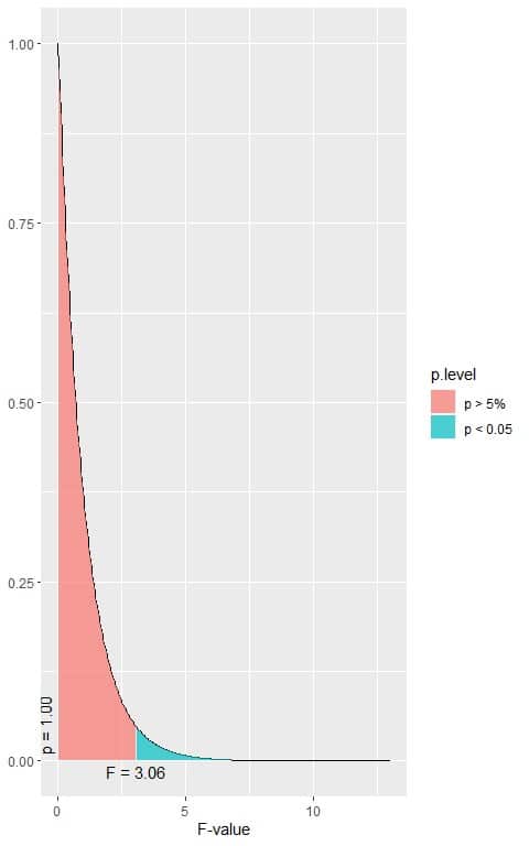
5. When the F-value = 3.06, the area to the right or the p-value < 0.05.

In our example, the F-value = 119.26 which is larger than 3.06, so the p-value is very much smaller than 0.05.

The p-value is < 0.05, so it is a statistically significant result and we reject the null hypothesis.

This means that there is a difference between at least two of the species in their sepal length mean.

Since we have 3 groups in our data, we cannot know which pair mean is significantly different from each other.

Previous Lesson | Main Page | Next Lesson