Approximating Integrals – Midpoint, Trapezoidal, and Simpson’s Rule

Approximating integrals are extremely helpful when we can’t evaluate a definite integral using traditional methods. Through numerical integration, we’ll be able to approximate the values of the definite integrals.

The techniques of approximating integrals will show us how it’s possible to numerically estimate the definite integral of any function. The three common numerical integration techniques are the midpoint rule, trapezoid rule, and Simpson’s rule.

At this point in our integral calculus discussion, we’ve learned about finding the indefinite and definite integrals extensive. There are instances, however, that finding the exact values of definite integrals won’t be possible. This is when approximating integrals enter.

In this article, we’ll focus on approximating integrals using the three mentioned techniques. Since we’re dealing with definite integrals, review your understanding of the fundamental theorem of calculus.

When to approximate an integral?      

We can approximate integrals by estimating the area under the curve of $\boldsymbol{f(x)}$ for a given interval, $\boldsymbol{[a, b]}$. In our discussion, we’ll cover three methods: 1) midpoint rule, 2) trapezoidal rule and 3) Simpson’s rule.

As we have mentioned, there are functions where finding their antiderivatives and the definite integrals will be an impossible feat if we stick with the analytical approach. This is when the three methods for approximating integrals will come in handy.

\begin{aligned}\int_{0}^{4} e^{x^2}\phantom{x}dx\\\int_{0}^{2} \dfrac{\sin x}{x}\phantom{x}dx \end{aligned}

These are two examples of definite integrals that will be challenging to evaluate if we use the integration techniques we’ve learned in the past.

This is when the three integral approximation techniques enter. The first approximation you’ll learn in your integral calculus classes is the Riemann sum. We’ve learned how it’s possible to estimate the area under the curve by dividing the region into smaller rectangles with a fixed width.

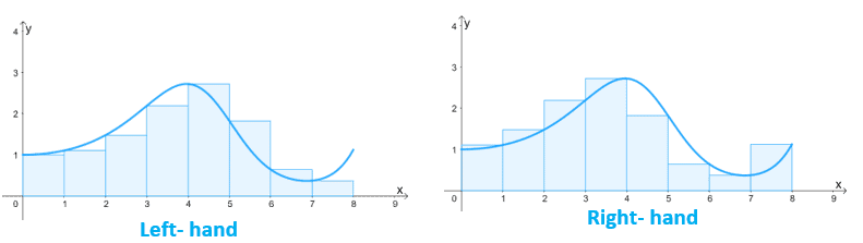
The graph shown above highlights how the Riemann sum works: divide the region under the curve with $n$ rectangles that share a common width, $\Delta x$. The value of $\Delta x$ is simply the difference between the intervals’ endpoints divided by $n$: $\Delta x = \dfrac{b- a}{n}$.

We can estimate the area and the integral using the relationships shown below:

Keep in mind the $x_i$ represents the initial value that we’re starting with. We’ve already discussed the Riemann sum in this article, so make sure to check it out in case you need a refresher.

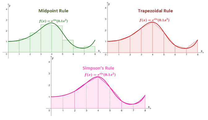
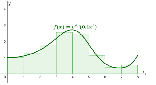
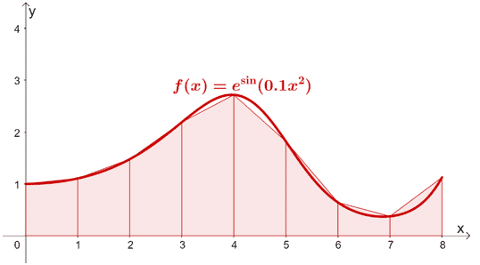
In the next section, we’ll show you the three numerical integration methods you can use to integrate complex integrals such as $f(x) = e^{\sin(0.1x^2)}$. We’ll also show you examples to make sure that we implement each technique.

How to approximate an integral?

The three approximation techniques that we’ll focus on using similar processes like that of the Riemann sum. We’ll show you what makes each technique special and of course, show you how to implement each method to approximate integrals.

Midpoint rule: integral approximation definition

It’s a good thing that we did a refresher on Riemann sum. That’s because the midpoint rule is an extension of the Riemann sum. The midpoint rule utilizes the two subinterval’s midpoint, $x_i$.

Let’s say we want to evaluate $\int_{a}^{b} f(x)\phantom{x} dx$, approximate its value using the midpoint rule by following the steps below:

• Divide the intervals into $n$ equal parts. Each new subinterval must have a width of $\Delta x = \dfrac{b – a}{n}$.
• We must begin with $x_0 = a$ and end with $x_n = b$. Meaning, we’ll have subintervals, $[x_0, x_1], [x_1, x_2], [x_2, x_3],…,[x_{n- 1}, x_n]$.
• Find the height of the rectangle formed by two subintervals, $x_{i-1}$ and $x_i$, by finding their midpoint: $\overline{x_i} = \dfrac{x_{i -1} + x_i}{2}$.
• Approximate the definite integral by finding the value of $\approx \sum_{i= 1}^{n} f(\overline{x_i}) \Delta x$

This means that through the midpoint rule, we can evaluate the definite integral using the formula shown below:

\begin{aligned}M_n &= \sum_{i =1}^{n}f(\overline{x_i})\Delta x\\\int_{a}^{b} f(x)\phantom{x}dx &= \lim_{n \rightarrow \infty} M_n\end{aligned}

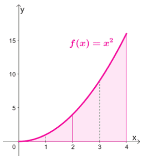
To better understand the midpoint rule’s process, let’s estimate the value of $\int_{0}^{4} x^2\phantom{x}dx$ using the midpoint rule:

• Divide the interval into four subintervals with a width of: $\Delta x = \dfrac{4 -0}{4} = 1$ unit.
• This means that we have the following intervals: $[0, 1]$, $[1, 2]$, $[2, 3]$, and $[3, 4]$.
• Find the respective midpoints shared by each pair of subintervals: $\left\{\dfrac{1}{2}, \dfrac{3}{2},\dfrac{5}{2},\dfrac{7}{2}\right\}$.

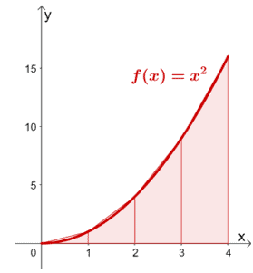
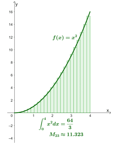
The graph below illustrates how the integral of $x^2$ is approximated using the midpoint rule.

Find the value of $\int_{0}^{4} x^2\phantom{x} dx$ by evaluating $\boldsymbol{f(x)}$ at the midpoints. Multiply each value to $\boldsymbol{\Delta x}$ then add all resulting values to estimate the integral’s value.

\begin{aligned}M_4 &= \sum_{i =1}^{4}f(\overline{x_i})\cdot (\Delta x) \\&= (1)f\left(\dfrac{1}{2}\right) + (1)f\left(\dfrac{3}{2}\right)+ (1)f\left(\dfrac{5}{2}\right) + (1)f\left(\dfrac{5}{2}\right)\\&= 1 \cdot \dfrac{1}{4}+ 1 \cdot \dfrac{9}{4} +1 \cdot \dfrac{25}{4}+ 1 \cdot \dfrac{49}{2} \\&= 21\end{aligned}

If we evaluate the integral, $\int_{0}^{4} x^2\phantom{x} dx$, it’s actual value will be $\dfrac{64}{3}$ or $21.\overline{3}$. This shows that the estimated value from the midpoint rule is actually close to the actual value.

Whenever possible, find the absolute error of the approximation by finding the absolute value of the difference between the integral’s actual value and approximated value.

\begin{aligned}\left|21 – \dfrac{64}{3}\right| &= \dfrac{1}{3}\\&\approx 0.33\end{aligned}

We can also find the relative error of the approximation by expressing the absolute error as the percent change of the actual value as shown below.

\begin{aligned}\left|\dfrac{A – B}{A}\right| \cdot 100\%\end{aligned}

This means that relative error for our calculation is:

\begin{aligned}\left|\dfrac{21 – \dfrac{64}{3}}{21}\right| \cdot 100\% &\approx 1.58\%\end{aligned}

These two error approximations confirm our observation: that the approximate value is a good enough estimation. Of course, it’s much easier to simply evaluate $\int_{0}^{4} x^2\phantom{x} dx$ analytically. But as we have mentioned, that won’t be the case for complex integrals.

Trapezoidal rule: integral approximation definition

For this method, instead of using rectangles, we’ll be using trapezoids. Hence, its name: trapezoidal rule. When given a definite integral, we can estimate the value of $\int_{a}^{b} f(x)\phantom{x}dx$ by approximating the area of the trapezoids under the curve.

The midpoint and trapezoid rules will have similar steps. Before we begin, recall that the formula for the trapezoid’s area is $\dfrac{1}{2}h(b_1 + b_2)$, where $h$ represents the height and $b_1$ and $b_2$ represents the two bases. Now, let’s go ahead and break down the steps for the trapezoid rule’s process:

• Divide the intervals of the given definite integral into $n$ equal parts. Determine the subinterval’s height by dividing $b -a$ by $n$: $\Delta x = \dfrac{b – a}{n}$.
• Keep in mind that we must have $x_0 = a$ and $x_n = b$. This means that the endpoints of the intervals are: $\{x_0, x_1, x_2, …, x_n\}$.
• Approximate the first trapezoid’s area using $f(x_0)$ and $f(x_1)$ as its bases.

\begin{aligned}T_1 &= \dfrac{1}{2}\Delta x [f(x_0) + f(x_1)]\end{aligned}

• Apply the same process to find the areas of the rest of the trapezoids then add up the areas for all $n$ trapezoids.

We’ll focus on the last bullet: adding up all the areas of the $n$ trapezoids. If we have the subinterval’s endpoints, $\{x_0, x_1, x_2, …, x_n\}$, we can find the sum of the areas, $T_n$, as shown below.

\begin{aligned}T_n &= \dfrac{\Delta x }{2}[f(x_0) + f(x_1)]+\dfrac{\Delta x }{2}[f(x_1) + f(x_2)]+ …+ \dfrac{\Delta x }{2}[f(x_{n-1}) + f(x_n)]\\&= \dfrac{\Delta x }{2}[f(x_0) + 2f(x_1)+ 2f(x_2)+ …+ 2f(x_{n -1})+ f(x_n)]\\\lim_{n\rightarrow +\infty}T_n &= \int_{a}^{b}f(x)\phantom{x}dx\end{aligned}

This means that we can estimate the definite integral by applying the formula for $T_n$ and that’s the Trapezoidal rule.

Estimate the value of $\int_{0}^{4} x^2\phantom{x}dx$ using the trapezoidal rule and four subintervals this time. Afterward, compare the approximate value of the integral and its actual value: $\dfrac{64}{3}$ squared units.

• Find each of the four trapezoids’ heights: $\Delta x = \dfrac{4 -0}{4} = 1$ unit.
• We’ll be working with four trapezoids with the following subintervals with the following endpoints: $\{0, 1, 2, 3,4\}$
• Calculate the areas of the trapezoids by evaluating functions at the endpoints.

Here’s the graph of $f(x) = x^2$ with the area under its curve is divided into four trapezoids. Calculate the total area of the four trapezoids as shown below:

\begin{aligned}T_4 &= \dfrac{\Delta x }{2}[f(x_0) + 2f(x_1)+ 2f(x_2)+ 2f(x_3)+ f(x_4)]\\&= \dfrac{1}{2}[f(0)+ 2f(1)+ 2f(2) + 2f(3)+ f(4)]\\&= \dfrac{1}{2}[0 + 2(1) + 2(4) + 2(9) + 16]\\&= 22\end{aligned}

Since $T_4 = 22$, $\int_{0}^{4} x^2\phantom{x}dx$ is approximately equal to $22$ squared units through the trapezoidal rule. As we did with the midpoint rule, let’s find our approximation’s absolute and relative error:

These two values show us that the value returned by trapezoidal rule is close enough compared to its actual value.

Simpson’s rule: integral approximation definition

Before we dive right into the process of Simpson’s rule, let’s first observe how the accuracies of midpoint and trapezoidal rules’ approximations improve as we use more intervals. 

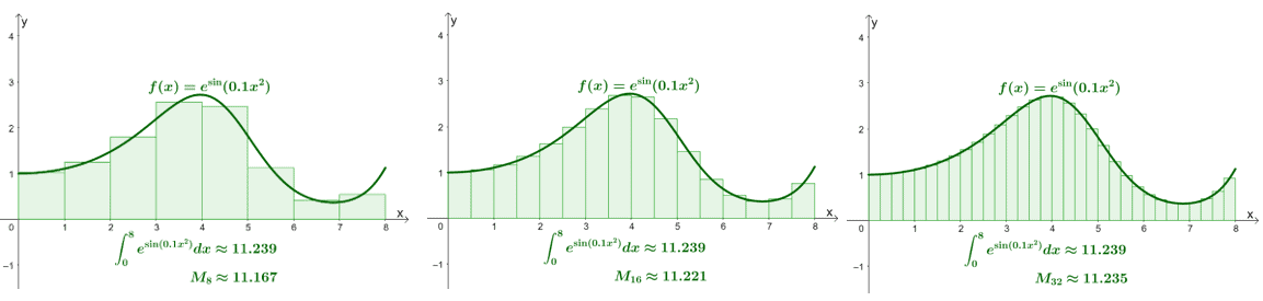
For the midpoint rule, we can see that we divide the regions into smaller rectangles, the approximations become closer to the definite integral’s value.

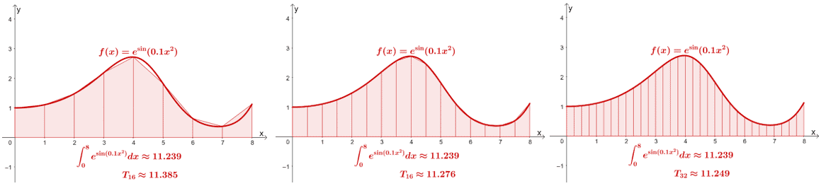
The same goes for the trapezoidal rule – the approximation becomes more accurate as we use more trapezoids. If we want a more accurate approximation, we’ll have to evaluate more values. That becomes problematic and time-consuming especially when we need to account for a certain error threshold.

This where Simpson’s rule comes in handy: this particular method utilizes quadratic curves instead. This is why Simpson’s rule returns more accurate approximations for functions with curves. The midpoint and trapezoidal rules, on the other hand, will return better results for straight lines.

In Simpson’s rule, we approximate the area under the curve by piecing together three quadratic curves within the set subinterval’s width. The more intervals (and consequently, more parabolic curves), the better the approximation.

This means that when we’re given $\int_{a}^{b}f(x) \phantom{x}dx$, we are approximating the area of the region bounded by $(a, f(a))$, $\left(\dfrac{a + b}{2}, f\left(\dfrac{a + b}{2}\right)\right)$, and $(b, f(b))$.

Let’s go ahead and break down the process of approximating $\int_{a}^{b}f(x) \phantom{x}dx$:

• Find the distance between each interval and express it as $\Delta x = \dfrac{b – a}{n}$.
• We’ll have the following endpoints for the $n$ subintervals: $\{x_0, x_1, x_2,…, x_n\}$.
• Approximate the definite integral using the formula for Simpson’s rule as shown below.

\begin{aligned}S_n &= \dfrac{\Delta x }{3}[f(x_0) + 4f(x_1)+ 2f(x_2)+ 4f(x_3)+ 2f(x_4)+ …+ 2f(x_{n -2})+4f(x_{n -1})+ f(x_n)]\\\lim_{n\rightarrow +\infty}S_n &= \int_{a}^{b}f(x)\phantom{x}dx\end{aligned}

This may form may look intimidating, but this is simply equivalent to finding the weighted average of the approximation returned by the midpoint and trapezoidal rule. It’s also equivalent to the average of the left and right-hand Riemann sums.

Why don’t we estimate $\int_{0}^{4}x^2 \phantom{x}dx$ using Simpson’s rule? We’re still using four intervals for our approximation.

• As with before, we have $\Delta x = \dfrac{4 -0}{4} = 1$ unit
• The area will have the following subintervals and endpoints: $\{0, 1, 2, 3,4\}$
• Apply the formula for Simpson’s rule to estimate the definite integral.

Let us show you the graph of $f(x)= x^2$ as well as the region’s area under the curve partitioned through Simpson’s rule.

What are the error bounds for the three methods?

In the previous examples, we’ve shown you how to compare the approximated and actual values of the definite integral. We can use the absolute and relative errors to gauge the accuracy of the three approximations.

Here’s the catch though: most of the time, we only use these approximations when we can’t evaluate the definite integral analytically. When this happens, we can still gauge the accuracy for the three approximations.

If we’re given a function, $f(x)$, that is continuous and twice differentiable over the interval, $[a,  b]$. Let $M$ represent the maximum value of $|f^{\prime\prime}(x)|$ over the interval, $[a, b]$. We can calculate the error bounds for the midpoint, trapezoidal, and the Simpson’s rule as shown below:

With these error bounds, we’ll now be able to know the value of $n$ to guarantee the accuracy of these estimated definite integrals.

Let’s say we want to find the right value of $n$ so that the approximated value of $\int_{0}^{4} x^2\phantom{x}dx$ is accurate within $0.01$. Assume that we’re using the midpoint rule.

Begin by finding the second derivative of $x^2$ then determine the second derivative’s maximum value.

\begin{aligned}\dfrac{d}{dx} x^2 &= 2x\\\dfrac{d}{dx} 2x &= 2\end{aligned}

Since the second derivative is equal to $2$, $M =2$. Use our given lower and upper limits, $a = 0$ and $b = 4$. Find the value of $n$ so that $M_n$ is less than or equal to $0.01$.

\begin{aligned}M_n &\leq 0.01\\\dfrac{M(b – a)^3}{24n^2}&\leq 0.01\\\dfrac{2(4 -0)^3}{24n^2}&\leq 0.01\\n &\geq \sqrt{\dfrac{2(64)}{24(0.01)}}\approx23.09\end{aligned}

This means that if we want to have an accuracy of at least $0.01$, $n$ must be equal to $23$.

This confirms that with $n =23$ or with $23$ rectangles, we can approximate $\int_{0}^{4} x^2 \phantom{x} dx$ up to a $0.01$ error.

Summary of the three methods used in approximating integrals

Before working on more examples, let us summarize our discussion for you first. Here’s a table summarizing the calculations needed for the midpoint, trapezoidal, and Simpson’s rules.

When we have the approximated and actual values, we can also check the approximations for absolute and relative errors.

Of course, if the actual value is not available, we can use the upper error bounds to find the right parameters for our approximation.

 Example 1

Given that $n =6$, estimate the value of $\int_{2}^{8} \dfrac{1}{x^2 + 1}\phantom{x}dx$ using the following approximating integral methods:

a. Midpoint Rule $(M_n)$
b. Trapezoidal Rule $(T_n)$
c. Simpson’s Rule $(S_n)$
Report your approximations to five decimal places.

Solution

To apply the midpoint rule for the given definite integral, find $\Delta x$ and the subintervals first:

• Using $n=6$, $a = 2$, and $b = 8$, we have $\Delta x=\dfrac{8 -2}{6} = 1$.
• The subintervals that we’ll be working with are :$[2, 3]$, $[3, 4]$, $[4,5]$, $[5,6]$, $[6,7]$, and $[7, 8]$.
• This means that we have the following midpoints, $\overline{x_i}: \left\{\dfrac{5}{2}, \dfrac{7}{2}, \dfrac{9}{2}, \dfrac{11}{2}, \dfrac{13}{2}, \dfrac{15}{2}\right\}$.

Apply the formula for the midpoint rule, $ M_n = \sum_{i =1}^{n}f(\overline{x_i})\Delta x$.

\begin{aligned}M_6 &= \sum_{i =1}^{6}f(\overline{x_i})\Delta x\\&= (1)f\left(\dfrac{5}{2}\right) +(1)f\left(\dfrac{7}{2}\right)+(1)f\left(\dfrac{9}{2}\right)\\&+(1)f\left(\dfrac{11}{2}\right)+(1)f\left(\dfrac{13}{2}\right) +(1)f\left(\dfrac{15}{2}\right)\\&=\dfrac{4}{29}+\dfrac{4}{53}+\dfrac{4}{85}+\dfrac{4}{125}+\dfrac{4}{173} + \dfrac{4}{229}\\&\approx 0.33305\end{aligned}

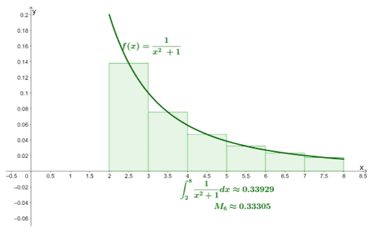
This means that with $n = 6$ as interval, $\int_{2}^{8}\dfrac{1}{x^2 +1}\phantom{x}dx$ is approximately equal to $0.33305$. We’ve included a graph to show you how this approximation would appear when plotted, but this is not a required step.

We’ll use the same values for $\Delta x$ and the subintervals to approximate the integral using the trapezoidal rule. Apply the formula below to approximate $\int_{2}^{8}\dfrac{1}{x^2 +1}\phantom{x}dx$.

\begin{aligned}T_n &= \dfrac{\Delta x }{2}[f(x_0) + 2f(x_1)+ 2f(x_2)+ …+ 2f(x_{n -1})+ f(x_n)]\end{aligned}

Evaluate $f(x)$ at the following endpoints: $\{2,3, 4, 5, 6, 7, 8\}$. Hence, we have the estimated value of $T_6$ as shown below.

\begin{aligned}T_6 &= \dfrac{\Delta x }{2}[f(x_0) + 2f(x_1)+ 2f(x_2)+ 2f(x_3)+2f(x_4)+2f(x_5)+ f(x_6)]\\&= \dfrac{1}{2}[f(2) + 2f(3)+ 2f(4)+ 2f(5)+2f(6)+2f(7)+ f(8)]\\&= \dfrac{1}{2}\left[\dfrac{1}{5} + \dfrac{1}{5} +\dfrac{2}{17}+\dfrac{1}{13}+\dfrac{2}{37}+\dfrac{1}{25}+\dfrac{1}{65}\right]\\&\approx 0.35200\end{aligned}

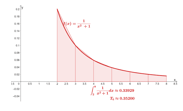
Through the trapezoidal rule, we have $\int_{2}^{8} \dfrac{1}{x^2 + 1}\phantom{x}dx$ as approximately $0.35200$.

Let’s now proceed approximating the integral using the Simpson’s rule. Apply the formula shown below to estimate $\int_{2}^{8} \dfrac{1}{x^2 + 1}\phantom{x} dx$.

\begin{aligned}S_n &= \dfrac{\Delta x }{3}[f(x_0) + 4f(x_1)+ 2f(x_2)+ 4f(x_3)+ 2f(x_4)+ …+ 2f(x_{n -2})+4f(x_{n -1})+ f(x_n)] \end{aligned}

Use the same values for $\Delta x$ and the endpoints.

\begin{aligned}S_6 &= \dfrac{\Delta x }{3}[f(x_0) + 4f(x_1)+ 2f(x_2)+ 4f(x_3)+ 4f(x_4)+ 2f(x_5)+ 4f(x_6)+ +f(x_7)]\\&=\dfrac{1 }{3}[f(2) + 4f(3)+ 2f(4)+ 4f(5)+ 2f(6)+ 4f(7)+ f(8)]\\&=\dfrac{1}{3}\left[\dfrac{1}{5} + \dfrac{2}{5}+\dfrac{2}{17}+\dfrac{2}{13}+\dfrac{2}{37}+\dfrac{2}{25}+ \dfrac{1}{65} \right ]\\&\approx 0.34031 \end{aligned}

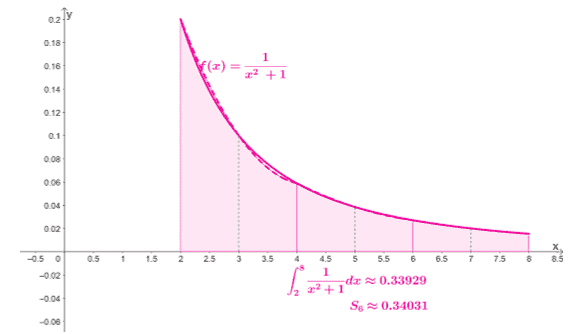
This confirms our result: $\int_{2}^{8} \dfrac{1}{x^2 + 1}\phantom{x} dx$ is approximately $0.34031$ through the Simpson’s rule.

Hence, we have the following results:

Example 2

Use the results from the previous example and construct a table comparing the absolute and relative errors for the three methods.

Use the actual value shown below:

 \begin{aligned}\int_{2}^{8} \dfrac{1}{x^2 + 1}\phantom{x}dx = \tan^{-1}(8) -\tan^{-1}(2) \approx 0.33929\end{aligned}

Solution

To estimate the absolute and relative errors, we’ll compare the actual value with the approximated values returned through the three methods: midpoint rule, trapezoidal rule, and Simpson’s rule.

Use the formula shown below and use replace $A$ with the actual value and $B$ with the approximated value.

Hence, we have the following absolute and relative errors for the three methods:

From this table of values, we can also see that the Simpson’s rule returned the smallest absolute and relative errors.

Practice Questions

1. Given that $n =6$, estimate the value of $\int_{2}^{8} \dfrac{1}{x^2 – 1}\phantom{x}dx$ using the following approximating integral methods:

a. Midpoint Rule $(M_n)$
b. Trapezoidal Rule $(T_n)$
c. Simpson’s Rule $(S_n)$
Report your approximations to five decimal places.

2. Given that $n =8$, estimate the value of $\int_{1}^{5} \dfrac{1}{e^x}\phantom{x}dx$ using the following approximating integral methods:

a. Midpoint Rule $(M_n)$
b. Trapezoidal Rule $(T_n)$
c. Simpson’s Rule $(S_n)$
Report your approximations to six decimal places.

3. Given that $n =5$, estimate the value of $\int_{0}^{4} \sqrt{e^x}\phantom{x}dx$ using the following approximating integral methods:

a. Midpoint Rule $(M_n)$
b. Trapezoidal Rule $(T_n)$
c. Simpson’s Rule $(S_n)$
Report your approximations to three decimal places.

4. Use the results from the previous example and construct a table comparing the absolute and relative errors for the three methods.
Use the actual value shown below:
\begin{aligned}\int_{0}^{4} \sqrt{e^x}\phantom{x}dx = 2(e^2 -1) \approx 12.778\end{aligned}

Answer Key

1.
a.$M_6 \approx 0.40784$
b.$T_6 \approx 0.45734$
c.$S_6 \approx 0.42434$
2.
a.$M_8 \approx 0.357407$
b.$T_8 \approx 0.368634$
c.$S_8 \approx 0.361149$
3.
a.$M_5 \approx 12.693 $
b.$T_5 \approx 12.948$
c.$S_5 \approx 12.779$
4.

Images/mathematical drawings are created with GeoGebra.