JUMP TO TOPIC
Class width – Explanation & Examples
 The definition of class width is:
“The class width is the difference between the upper or lower class limits of consecutive classes in a bin frequency table”.
In this topic, we will discuss the class width from the following aspects:
- What is the class width?
- How to find the class width?
- Class width formula.
- Role of class width.
- Practical questions.
- Answers.
What is the class width?
The class width is the difference between the upper or lower class limits of consecutive classes in a bin frequency table.
The bin frequency table groups values into equal-sized bins or classes and each class includes a range of values.
The frequency of each class is the number of data points it has.
The boundaries of each class are called the lower-class limit and the upper-class limit, and the class width is the difference between the lower (or higher) limits of successive classes.
All classes should have the same width.
How to find the class width?
We will go through an example for illustration.
Example 1
The following is the age (in years) of 50 participants from a certain survey.
participant | Age |
1 | 70 |
2 | 56 |
3 | 37 |
4 | 69 |
5 | 70 |
6 | 40 |
7 | 66 |
8 | 53 |
9 | 43 |
10 | 70 |
11 | 54 |
12 | 42 |
13 | 54 |
14 | 48 |
15 | 68 |
16 | 48 |
17 | 42 |
18 | 35 |
19 | 72 |
20 | 70 |
21 | 70 |
22 | 48 |
23 | 56 |
24 | 74 |
25 | 57 |
26 | 52 |
27 | 58 |
28 | 62 |
29 | 56 |
30 | 68 |
31 | 70 |
32 | 46 |
33 | 35 |
34 | 56 |
35 | 50 |
36 | 48 |
37 | 47 |
38 | 60 |
39 | 63 |
40 | 71 |
41 | 43 |
42 | 65 |
43 | 38 |
44 | 64 |
45 | 73 |
46 | 54 |
47 | 67 |
48 | 58 |
49 | 62 |
50 | 70 |
What is the proper class width for a bin frequency table of this data?
- Determine the number of bins or classes you need.
There are no hard rules about how many bins to pick, but there are some general guidelines:
- Pick between 5 and 20 classes.
- Make sure you have a few items in each bin. For example, if you have 40 data points, you can choose 5 bins (8 data points per category), but not 20 bins (which would give you only 2 data points per bin).
- Use the mathematical formula to choose the number of classes.
The formula is log(number of observations)/ log(2). You would round up the answer to the next integer.
For this data, log(50)/log(2) = 5.6 will be rounded up to become 6, so the number of classes should be 6.
- Sort the data and subtract the minimum data value from the maximum data value to get the data range.
35 35 37 38 40 42 42 43 43 46 47 48 48 48 48 50 52 53 54 54 54 56 56 56 56 57 58 58 60 62 62 63 64 65 66 67 68 68 69 70 70 70 70 70 70 70 71 72 73 74.
In our age list, the minimum value is 35 and the maximum value is 74, so the data range = 74 – 35 = 39.
- Divide the data range in Step 2 by the number of classes you get in Step 1.
Round the number you get up to a whole number to get the class width.
Class width = 39 / 6 = 6.5. Rounded up to 7.
- Add the class width, 7, sequentially (6 times because we have 6 bins) to the minimum value to create the different 6 classes.
35 + 7 = 42 so the first class is 35-42.
42+7 = 49 so the next bin is 42-49.
49+7 = 56, so the next bin is 49-56.
56+7 = 63, so the next bin is 56-63.
63+7 = 70, so the next bin is 63-70.
70+7 = 77, so the next bin is 70-77.
- We draw a table of 2 columns. The first column carries the different classes of the data that we created in step 4.
The second column contains the frequency of age values in each class.
range | frequency |
35 – 42 | 7 |
42 – 49 | 8 |
49 – 56 | 10 |
56 – 63 | 7 |
63 – 70 | 14 |
70 – 77 | 4 |
We see that:
- The age bin “35-42” contains the ages from 35 to 42.
- The next age bin “42-49” contains the ages larger than 42 till 49, and so on.
- The class width is 7 for any two consecutive classes.
- For example, the first class is 35-42 with 35 as the lower limit and 42 as the upper limit. The next class is 42-49 with 42 as the lower limit and 49 as the upper limit. The class width = 42-35 = 49-42 = 7.
- If you sum these frequencies, you will get 50 which is the total number of data. 7+8+10+7+14+4 = 50.
We can then use this bin frequency table to plot a histogram of this data where we plot the data bins on a certain axis against their frequency on the other axis.
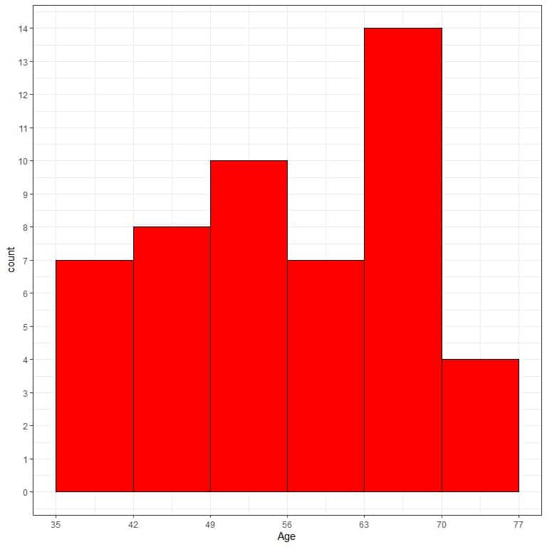
We see that the most frequent bin is the 63-70 bin with 14 occurrences.
We see also that the data is somewhat left-skewed.
Class width formula
From the above example, we see that the class width formula:
class width = data range/number of classes = (maximum – minimum)/number of classes
Role of class width
By selecting the suitable class width according to the above guidelines, we can observe the data distribution.
Selecting too tight or too wide class width can result in poor representation of data distribution.
Example 1
The following bin frequency table is for the age (in years) of 21407 participants from a certain survey.
The suitable number of classes = log(21407)/log(2) = 14.39 or 15.
Data range = 89-18 = 71.
class width = 71/15 = 4.7 or 5.
range | frequency |
18 – 23 | 1528 |
23 – 28 | 1912 |
28 – 33 | 2086 |
33 – 38 | 2134 |
38 – 43 | 2154 |
43 – 48 | 2117 |
48 – 53 | 2033 |
53 – 58 | 1783 |
58 – 63 | 1570 |
63 – 68 | 1219 |
68 – 73 | 961 |
73 – 78 | 817 |
78 – 83 | 585 |
83 – 88 | 360 |
88 – 93 | 148 |
and plot this bin frequency table as a histogram.
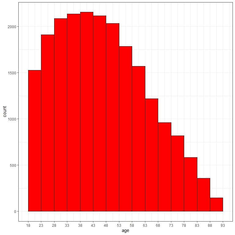
We see that the most frequent bin is the 38-43 bin with 2154 occurrences.
We see also that the data is somewhat right-skewed.
If we use too tight class width as 2, we will get the following frequency table.
range | frequency |
18 – 20 | 591 |
20 – 22 | 576 |
22 – 24 | 705 |
24 – 26 | 796 |
26 – 28 | 772 |
28 – 30 | 809 |
30 – 32 | 852 |
32 – 34 | 850 |
34 – 36 | 845 |
36 – 38 | 864 |
38 – 40 | 867 |
40 – 42 | 839 |
42 – 44 | 880 |
44 – 46 | 826 |
46 – 48 | 859 |
48 – 50 | 847 |
50 – 52 | 790 |
52 – 54 | 783 |
54 – 56 | 749 |
56 – 58 | 647 |
58 – 60 | 661 |
60 – 62 | 617 |
62 – 64 | 545 |
64 – 66 | 490 |
66 – 68 | 476 |
68 – 70 | 414 |
70 – 72 | 395 |
72 – 74 | 332 |
74 – 76 | 350 |
76 – 78 | 287 |
78 – 80 | 262 |
80 – 82 | 224 |
82 – 84 | 199 |
84 – 86 | 149 |
86 – 88 | 111 |
88 – 90 | 148 |
We see that the frequency table becomes too long with more than 20 bins and hard to grasp to get the data distribution.
If we plot this bin frequency table as a histogram.
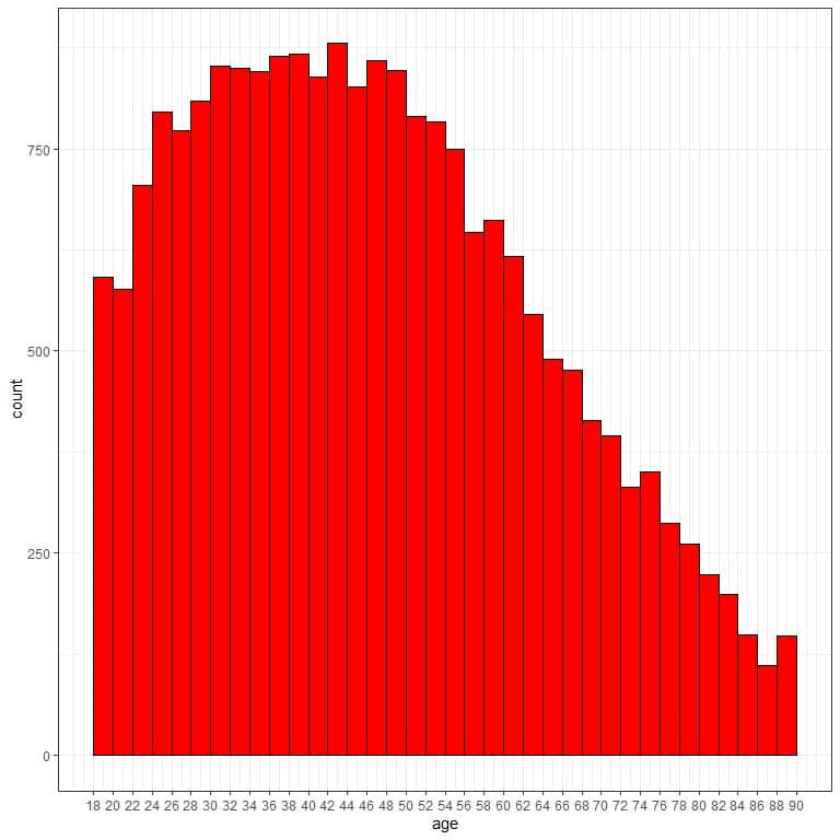
There are too many bins or classes and the data distribution is hard to see.
If we use a too wide class width of 36, we will get the following frequency table.
range | frequency |
18 – 54 | 14351 |
54 – 90 | 7056 |
We see that the frequency table with 2 bins only, and hard to grasp to get the data distribution.
If we plot this bin frequency table as a histogram.
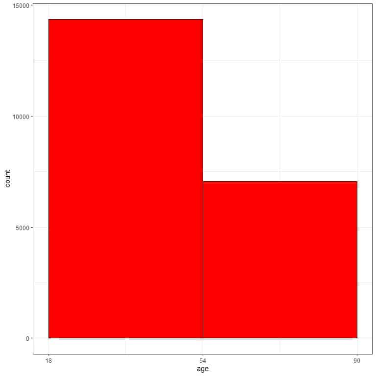
With only two bins, we have no idea about the data distribution.
Example 2
The following bin frequency table is for the physical activity (in Kcal/week) of 2206 participants from a certain survey.
The suitable number of classes = log(2206)/log(2) = 11.1 or 12.
Data range = 5083.2-0 = 5083.2.
class width = 5083.2/12 = 423.6 or 424.
range | frequency |
0 – 424 | 1442 |
424 – 848 | 563 |
848 – 1272 | 145 |
1272 – 1696 | 26 |
1696 – 2120 | 19 |
2120 – 2544 | 2 |
2544 – 2968 | 2 |
2968 – 3392 | 2 |
3392 – 3816 | 2 |
3816 – 4240 | 2 |
4240 – 4664 | 0 |
4664 – 5088 | 1 |
and plot this bin frequency table as a histogram.
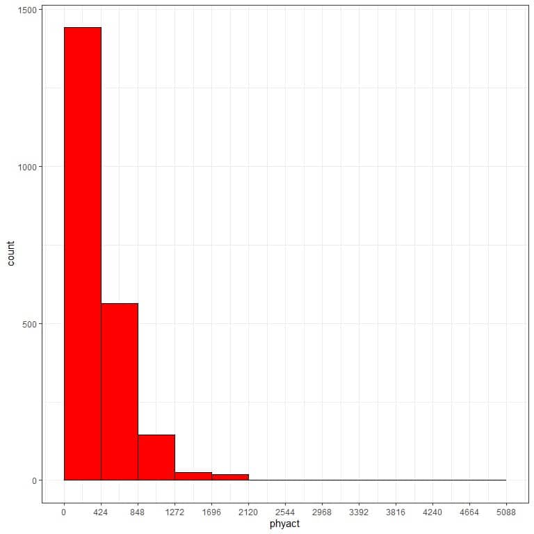
We see that the most frequent bin is the 0-424 bin with 1442 occurrences.
We see also that the data is somewhat right-skewed.
If we use too tight class width of 100, we will get the following frequency table.
range | frequency |
0 – 100 | 335 |
100 – 200 | 373 |
200 – 300 | 380 |
300 – 400 | 288 |
400 – 500 | 239 |
500 – 600 | 155 |
600 – 700 | 121 |
700 – 800 | 84 |
800 – 900 | 57 |
900 – 1000 | 48 |
1000 – 1100 | 33 |
1100 – 1200 | 30 |
1200 – 1300 | 9 |
1300 – 1400 | 9 |
1400 – 1500 | 4 |
1500 – 1600 | 7 |
1600 – 1700 | 4 |
1700 – 1800 | 9 |
1800 – 1900 | 6 |
1900 – 2000 | 3 |
2000 – 2100 | 1 |
2100 – 2200 | 0 |
2200 – 2300 | 1 |
2300 – 2400 | 0 |
2400 – 2500 | 1 |
2500 – 2600 | 0 |
2600 – 2700 | 1 |
2700 – 2800 | 1 |
2800 – 2900 | 0 |
2900 – 3000 | 0 |
3000 – 3100 | 0 |
3100 – 3200 | 1 |
3200 – 3300 | 1 |
3300 – 3400 | 0 |
3400 – 3500 | 1 |
3500 – 3600 | 0 |
3600 – 3700 | 0 |
3700 – 3800 | 1 |
3800 – 3900 | 0 |
3900 – 4000 | 0 |
4000 – 4100 | 0 |
4100 – 4200 | 0 |
4200 – 4300 | 2 |
4300 – 4400 | 0 |
4400 – 4500 | 0 |
4500 – 4600 | 0 |
4600 – 4700 | 0 |
4700 – 4800 | 0 |
4800 – 4900 | 0 |
4900 – 5000 | 0 |
5000 – 5100 | 1 |
We see that the frequency table becomes too long with more than 20 bins and hard to interpret to get the data distribution.
If we plot this bin frequency table as a histogram.
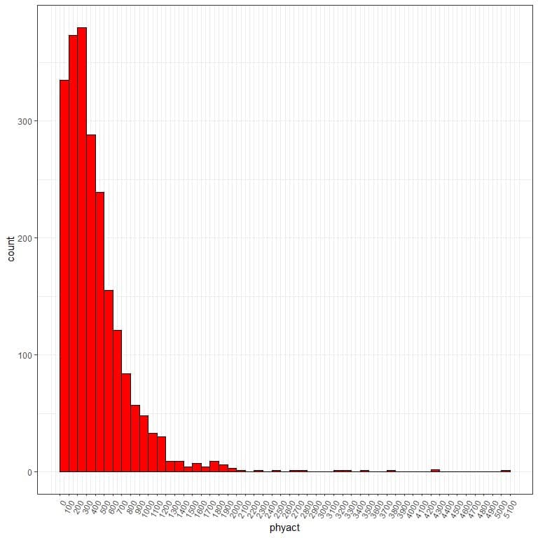
There are too many bins or classes and the class width is hard to see.
If we use too wide class width as 2600, we will get the following frequency table.
range | frequency |
0 – 2600 | 2197 |
2600 – 5200 | 9 |
We see that the frequency table is with 2 bins only, and hard to grasp to get the data distribution.
If we plot this bin frequency table as a histogram.
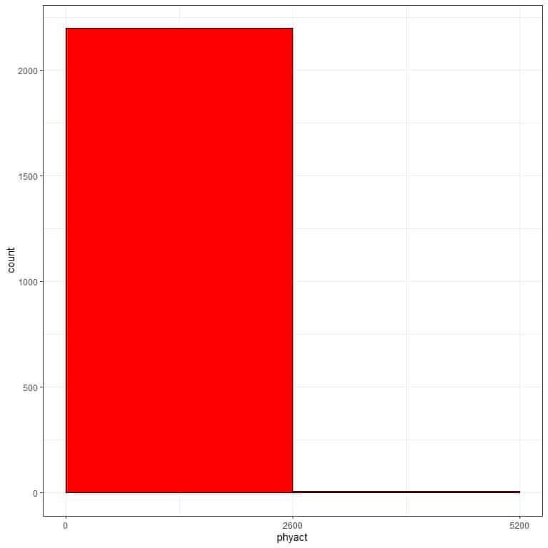
With only two bins, we have no idea about the data distribution.
Practical questions
- The following information is related to some price data.
The number of observations = 53940.
Minimum = $326.
Maximum = $18823.
What is the suitable class width for this data?
- The following information is related to some diamond weights.
The number of observations = 53940.
Minimum = 0.2 grams.
Maximum = 5.01 grams.
What is the suitable class width for this data?
- The following bin frequency table is for the wind speed of some storms (in knots).
range | frequency |
10 – 21 | 287 |
21 – 32 | 2258 |
32 – 43 | 1727 |
43 – 54 | 1575 |
54 – 65 | 1678 |
65 – 76 | 812 |
76 – 87 | 492 |
87 – 98 | 402 |
98 – 109 | 242 |
109 – 120 | 329 |
120 – 131 | 117 |
131 – 142 | 52 |
142 – 153 | 32 |
153 – 164 | 7 |
What is the most frequent bin?
Is this data skewed data?
- The following is the bin frequency table for some Ozone measurements.
range | frequency |
1 – 57 | 83 |
57 – 113 | 28 |
113 – 169 | 5 |
Is the class width suitable for this data?
Can you determine a more suitable number of classes for this data?
- The following is the bin frequency table for some solar radiation measurements.
range | frequency |
0 – 100 | 34 |
100 – 200 | 37 |
200 – 300 | 66 |
300 – 400 | 9 |
400 – 500 | 0 |
500 – 600 | 0 |
600 – 700 | 0 |
700 – 800 | 0 |
800 – 900 | 0 |
900 – 1000 | 0 |
What is wrong with this table?
Can you determine a more appropriate class width if you know that the data range is 327?
Answers
- The recommended number of bins or classes = log(53940)/log(2) = 15.7 rounded up to 16.
The data range = 18823-326 = 18497.
The class width = 18497/16 = 1156.062 rounded up to 1157.
- The recommended number of bins or classes = log(53940)/log(2) = 15.7 rounded up to 16.
The data range = 5.01-0.2 = 4.81.
The class width = 4.81/16 = 0.300625 rounded up to 0.31.
- The most frequent bin is “21-32” with 2258 occurrences.
This data is right-skewed because it is clustered at small values and large values have a much lower frequency.
- There are only 3 classes while there should be 5-20 classes.
The suitable number of classes = log(number of observations)/log(2) = log(83+28+5)/log(2) = 6.86 rounded up to 7.
- The bin frequency table has many empty bins at its end. These can be deleted to not confuse the reader and the table should be:
range | frequency |
0 – 100 | 34 |
100 – 200 | 37 |
200 – 300 | 66 |
300 – 400 | 9 |
The recommended number of bins or classes = log(34+37+66+9)/log(2) = 7.19 rounded up to 8.
The data range = 327.
The suitable class width = 327/8 = 40.88 rounded up to 41.